Unit - 4
LinkedList and Tree
4.1.1 Concept of LinkedList
A Linked List is a collection of objects called nodes that are kept in memory at random. A node has two fields: data saved at that specific address and a pointer to the next node in the memory. The list's last node has a pointer to the null.
The following are some key terms to know in order to grasp the notion of Linked List.
● Link − A linked list's links can each store a piece of data known as an element.
● Next − Each link in a linked list has a Next link that points to the next link.
● LinkedList − A Linked List has the connecting link to the initial link, which is referred to as First.

Fig 1: Linked list
Uses of Linked List
● The list does not have to be kept in order in the memory. The node can be located anywhere in memory and linked to form a list. This results in optimal space usage.
● The list size is restricted by memory and does not need to be announced ahead of time.
● The linked list cannot include an empty node.
● In a singly linked list, we can store values of primitive types or objects.
Advantages of Linked list
The following are some of the benefits of using a linked list:
● Dynamic data structure - The linked list's size can vary depending on the requirements. The size of a linked list is not fixed.
● Insertion and deletion - In contrast to arrays, insertion and deletion are much easier in linked lists. The items of an array are stored in a sequential order, whereas the elements of a linked list are stored in a random order. To add or remove an element from an array, we must first shift the elements to make room. Instead of shifting, we only need to update the address of the node's pointer in a linked list.
● Memory efficient - Because the size of a linked list can be adjusted to meet the needs, memory consumption in linked lists is low.
● Implementation - Linked lists can be used to implement both stacks and queues.
Disadvantages of Linked list
The following are some of the drawbacks of utilizing a linked list:
● Memory usage - Node takes up more memory than array in a linked list. Each node in the linked list has two sorts of variables, one of which is a simple variable and the other of which is a pointer variable.
● Traversal - The linked list makes traversal difficult. If we need to access an element in a linked list, we can't do so randomly, but an array can be accessed randomly by index. For example, if we want to go to the third node, we must first go through all of the nodes that come before it. As a result, accessing a certain node takes a long time.
● Reverse traversing - In a linked list, backtracking or reverse traversing is tough. The back pointer is easier to keep in a doubly-linked list, but it takes up more memory.
Program to create simple linked list
#include <iostream>
Using namespace std;
Struct Node {
Int data;
Struct Node *next;
};
Struct Node* head = NULL;
Void insert(int new_data) {
Struct Node* new_node = (struct Node*) malloc(sizeof(struct Node));
New_node->data = new_data;
New_node->next = head;
Head = new_node;
}
Void display() {
Struct Node* ptr;
Ptr = head;
While (ptr != NULL) {
Cout<< ptr->data <<" ";
Ptr = ptr->next;
}
}
Int main() {
Insert(3);
Insert(1);
Insert(7);
Insert(2);
Insert(9);
Cout<<"The linked list is: ";
Display();
Return 0;
}
Output:
The linked list is: 9 2 7 1 3
Key takeaway
A Linked List is a collection of objects called nodes that are kept in memory at random. A node has two fields: data saved at that specific address and a pointer to the next node in the memory. The list's last node has a pointer to the null.
4.1.2 Memory representation of LinkedList
● INFO and LINK are two arrays that can be used to represent linked lists, with INFO[K] and LINK[K] containing element and next node addresses, respectively.
● The list also needs a variable called 'Name' or 'Start,' which provides the first node's address. The last node's pointer field is NULL, indicating the end of the list. The example below illustrates how a linked list is stored in memory. The list's nodes do not have to be adjacent elements in the arrays INFO and LINK, and many lists can be stored in the same linear arrays INFO and LINK. However, each list must have a pointer variable that points to the first node.
● The linked list can be represented in memory as -
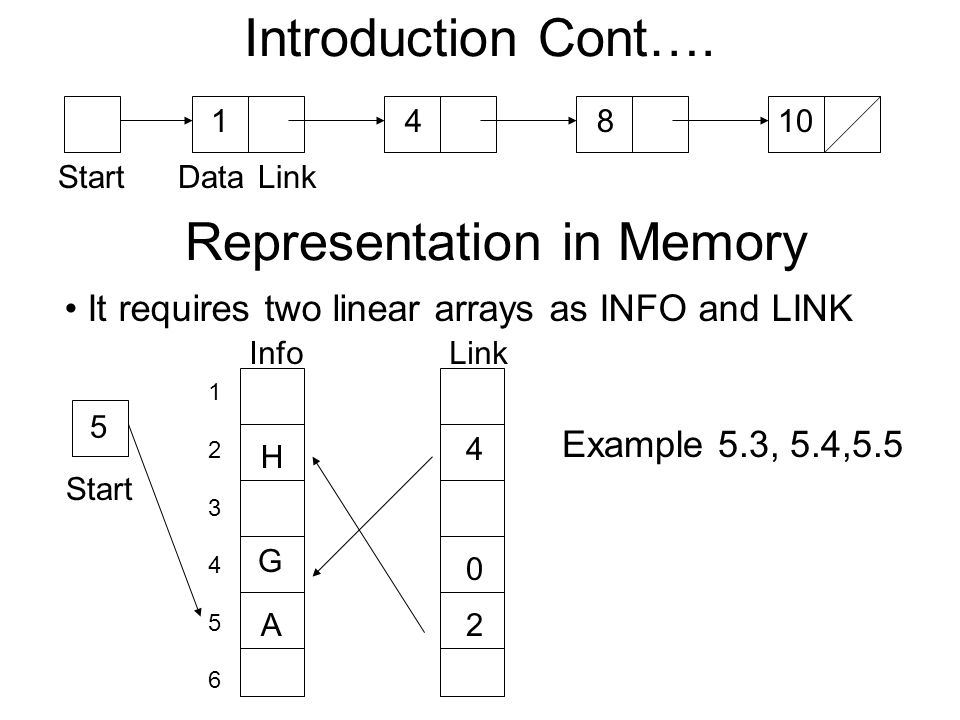
Fig 2: Example
4.1.3 Operations on LinkedList (Insertion, Deletion, Display and Search)
Insertion
When placing a node into a linked list, there are three possible scenarios:
● Insertion at the beginning
● Insertion at the end. (Append)
● Insertion after a given node
Insertion at the beginning
There's no need to look for the end of the list. If the list is empty, the new node becomes the list's head. Otherwise, we must connect the new node to the existing list's head and make the new node the list's head.
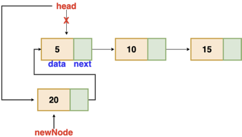
Fig 3: Insertion at beginning
// function is returning the head of the singly linked-list
Node insertAtBegin(Node head, int val)
{
newNode = new Node(val) // creating new node of linked list
if(head == NULL) // check if linked list is empty
return newNode
else // inserting the node at the beginning
{
newNode.next = head
return newNode
}
}
Insertion at the end
We'll go through the list till we reach the last node. The new node is then appended to the end of the list. It's worth noting that there are some exceptions, such as when the list is empty.
We will return the updated head of the linked list if the list is empty, because the inserted node is both the first and end node of the linked list in this case.
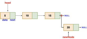
Fig 4: Insertion at end
// the function is returning the head of the singly linked list
Node insertAtEnd(Node head, int val)
{
if( head == NULL ) // handing the special case
{
newNode = new Node(val)
head = newNode
return head
}
Node temp = head
// traversing the list to get the last node
while( temp.next != NULL )
{
temp = temp.next
}
newNode = new Node(val)
temp.next = newNode
return head
}
Insertion after a given node
The reference to a node is passed to us, and the new node is put after it.
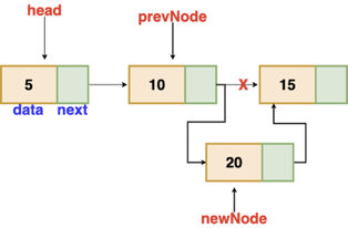
Fig 5: Insertion after given node
Void insertAfter(Node prevNode, int val)
{
newNode = new Node(val)
newNode.next = prevNode.next
prevNode.next = newNode
}
Deletion
These are the procedures to delete a node from a linked list.
● Find the previous node of the node to be deleted.
● Change the next pointer of the previous node
● Free the memory of the deleted node.
There is a specific circumstance in which the first node is removed upon deletion. We must update the connected list's head in this case.

Fig 6: Deleting a node in linked list
// this function will return the head of the linked list
Node deleteLL(Node head, Node del)
{
if(head == del) // if the node to be deleted is the head node
{
return head.next // special case for the first Node
}
Node temp = head
while( temp.next != NULL )
{
if(temp.next == del) // finding the node to be deleted
{
temp.next = temp.next.next
delete del // free the memory of that Node
return head
}
temp = temp.next
}
return head // if no node matches in the Linked List
}
Display
The print procedure is used to print the information for each node. This command displays the entire list.
Search
● In a linked list, the search operation is used to locate a certain entry.
● On a linked list structure, the most common search is sequential search.
● If the element is located, the search procedure is declared successful.
● The search will fail if the element is not found.
// Search a node
Bool searchNode(struct Node** head_ref, int key) {
struct Node* current = *head_ref;
while (current != NULL) {
if (current->data == key) return true;
current = current->next;
}
return false;
}
Key takeaway
- There's no need to look for the end of the list. If the list is empty, the new node becomes the list's head.
- The goal is to work your way through the list from start to finish. We might want to print the list or search for a certain node in it.
4.1.4 Types of LinkedList: Singly, Doubly LinkedList & Circular LinkedList
In programming, it is the most widely used linked list. When we talk about a linked list, we're talking about a singly linked list. The singly linked list is a data structure that is divided into two parts: the data portion and the address part, which contains the address of the next or successor node. A pointer is another name for the address component of a node.
Assume we have three nodes with addresses of 100, 200, and 300, respectively. The following diagram depicts the representation of three nodes as a linked list:

Fig 7: Singly linked list
In the diagram above, we can see three separate nodes with addresses of 100, 200, and 300, respectively. The first node has the address of the next node, which is 200, the second has the address of the last node, which is 300, and the third has the NULL value in its address portion because it does not point to any node. A head pointer is a pointer that stores the address of the first node.
Because there is just one link in the linked list depicted in the figure, it is referred to as a singly linked list. Just forward traversal is permitted in this list; we can't go backwards because there is only one link in the list.
Representation of the node in a singly linked list
Struct node
{
int data;
struct node *next;
}
In the above diagram, we've constructed a user-made structure called a node, which has two members: one is data of integer type, and the other is the node type's pointer (next).
Example
#include <iostream>
Using namespace std;
Struct Node {
int data;
struct Node *next;
};
Struct Node* head = NULL;
Void insert(int new_data) {
struct Node* new_node = (struct Node*) malloc(sizeof(struct Node));
new_node->data = new_data;
new_node->next = head;
head = new_node;
}
Void display() {
struct Node* ptr;
ptr = head;
while (ptr != NULL) {
cout<< ptr->data <<" ";
ptr = ptr->next;
}
}
Int main() {
insert(3);
insert(1);
insert(7);
insert(2);
insert(9);
cout<<"The linked list is: ";
display();
return 0;
}
Output
The linked list is: 9 2 7 1 3
Doubly linked list
The doubly linked list, as its name implies, has two pointers. The doubly linked list can be described as a three-part linear data structure: the data component, the address part, and the other two address parts. A doubly linked list, in other terms, is a list with three parts in each node: one data portion, a pointer to the previous node, and a pointer to the next node.
Let's pretend we have three nodes with addresses of 100, 200, and 300, respectively. The representation of these nodes in a doubly-linked list is shown below:

Fig 8: Doubly linked list
The node in a doubly-linked list contains two address portions, as shown in the diagram above; one part keeps the address of the next node, while the other half stores the address of the previous node. The address component of the first node in the doubly linked list is NULL, indicating that the prior node's address is NULL.
Representation of the node in a doubly linked list
Struct node
{
int data;
struct node *next;
Struct node *prev;
}
In the above representation, we've constructed a user-defined structure called a node, which has three members: one is data of integer type, and the other two are pointers of the node type, i.e. next and prev. The address of the next node is stored in the next pointer variable, whereas the address of the previous node is stored in the prev pointer variable. The type of both the pointers, i.e., next and prev is struct node as both the pointers are storing the address of the node of the struct node type.
Example
#include <iostream>
Using namespace std;
Struct Node {
int data;
struct Node *prev;
struct Node *next;
};
Struct Node* head = NULL;
Void insert(int newdata) {
struct Node* newnode = (struct Node*) malloc(sizeof(struct Node));
newnode->data = newdata;
newnode->prev = NULL;
newnode->next = head;
if(head != NULL)
head->prev = newnode ;
head = newnode;
}
Void display() {
struct Node* ptr;
ptr = head;
while(ptr != NULL) {
cout<< ptr->data <<" ";
ptr = ptr->next;
}
}
Int main() {
insert(3);
insert(1);
insert(7);
insert(2);
insert(9);
cout<<"The doubly linked list is: ";
display();
return 0;
}
Output
The doubly linked list is: 9 2 7 1 3
Circular linked list
A singly linked list is a type of circular linked list. The sole difference between a singly linked list and a circular linked list is that the last node in a singly linked list does not point to any other node, therefore its link portion is NULL. The circular linked list, on the other hand, is a list in which the last node connects to the first node, and the address of the first node is stored in the link section of the last node.
There are no nodes at the beginning or finish of the circular linked list. We can travel in either way, backwards or forwards. The following is a diagrammatic illustration of the circular linked list:
Struct node
{
int data;
struct node *next;
}
A circular linked list is a collection of elements in which each node is linked to the next and the last node is linked to the first. The circular linked list will be represented similarly to the singly linked list, as demonstrated below:
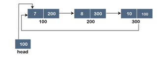
Fig 9: Circular linked list
Example
#include <iostream>
Using namespace std;
Struct Node {
int data;
struct Node *next;
};
Struct Node* head = NULL;
Void insert(int newdata) {
struct Node *newnode = (struct Node *)malloc(sizeof(struct Node));
struct Node *ptr = head;
newnode->data = newdata;
newnode->next = head;
if (head!= NULL) {
while (ptr->next != head)
ptr = ptr->next;
ptr->next = newnode;
} else
newnode->next = newnode;
head = newnode;
}
Void display() {
struct Node* ptr;
ptr = head;
do {
cout<<ptr->data <<" ";
ptr = ptr->next;
} while(ptr != head);
}
Int main() {
insert(3);
insert(1);
insert(7);
insert(2);
insert(9);
cout<<"The circular linked list is: ";
display();
return 0;
}
Output
The circular linked list is: 9 2 7 1 3
Key takeaway
- The singly linked list is a data structure that is divided into two parts: the data portion and the address part, which contains the address of the next or successor node.
- A pointer is another name for the address component of a node.
- The doubly linked list can be described as a three-part linear data structure: the data component, the address part, and the other two address parts.
- The circular linked list, on the other hand, is a list in which the last node connects to the first node, and the address of the first node is stored in the link section of the last node.
4.2.1 Concept of Tree, Tree terminology (root, child, parent, sibling, descendent, ancestor, leaf/external node, branch node/internal node, degree, edge, path, level, depth, height of node, height of tree, forest)
● A tree data structure is made up of nodes, which are items or entities that are joined together to represent or simulate hierarchy.
● Because it does not store data in a sequential order, a tree data structure is a non-linear data structure. Because the pieces in a Tree are grouped at numerous levels, it is a hierarchical structure.
● The root node in a Tree data structure is the topmost node. Each node has some data, which can be of any kind. Because the node in the above tree structure contains the employee's name, the data type is a string.
● Each node includes data as well as a link or reference to other nodes known as children.
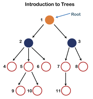
Fig 10: Tree
Each node in the above structure is labeled with a number. Each arrow in the diagram above represents a link between the two nodes.
Root - In a tree hierarchy, the root node is the highest node. To put it another way, the root node is the one that has no children. The root node of the tree is numbered 1 in the above structure. A parent-child relationship exists when one node is directly linked to another node.
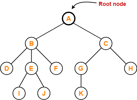
Fig 11: Example
Child node - If a node is a descendant of another node, it is referred to as a child node.

Parent - If a node has a sub-node, the parent of that sub-node is said to be that node.

Sibling - Sibling nodes are those that have the same parent.
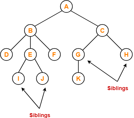
Descendant node - A descendant of a node is the direct successor of the supplied node. In the diagram above, node 10 is a descendent of node 5.
Ancestor node - Any previous node on a path from the root to that node is an ancestor of that node. There are no ancestors for the root node. Nodes 1, 2, and 5 are the ancestors of node 10 in the tree depicted above.
Leaf node - A leaf node is a node in the tree that does not have any descendant nodes. A leaf node is the tree's bottommost node. In a generic tree, there can be any number of leaf nodes. External nodes are also known as leaf nodes.
Internal node - An internal node is a node that has at least one child node.
Degree - The total number of branches of a node determines its degree. The highest degree of a node among all the nodes in the tree is called the tree's degree.

Edge - The edge is the connecting link between any two nodes. There are exactly (n-1) number of edges in a tree with n nodes.
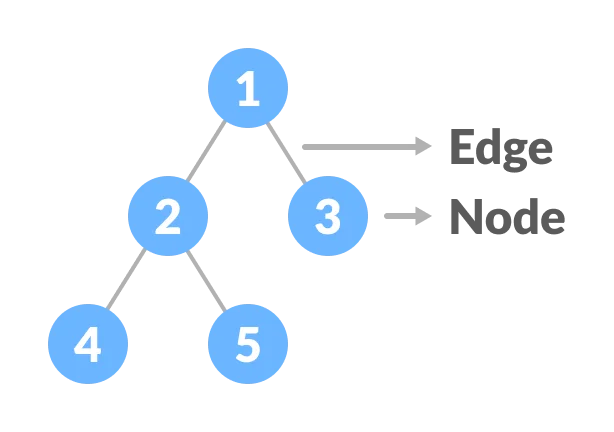
Path - Each arrow in the diagram above represents a link between the two nodes.
Level - Each step from the top to the bottom of a tree is referred to as a tree level. At each level or step, the level count starts at 0 and increases by one.
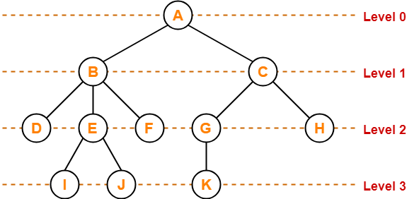
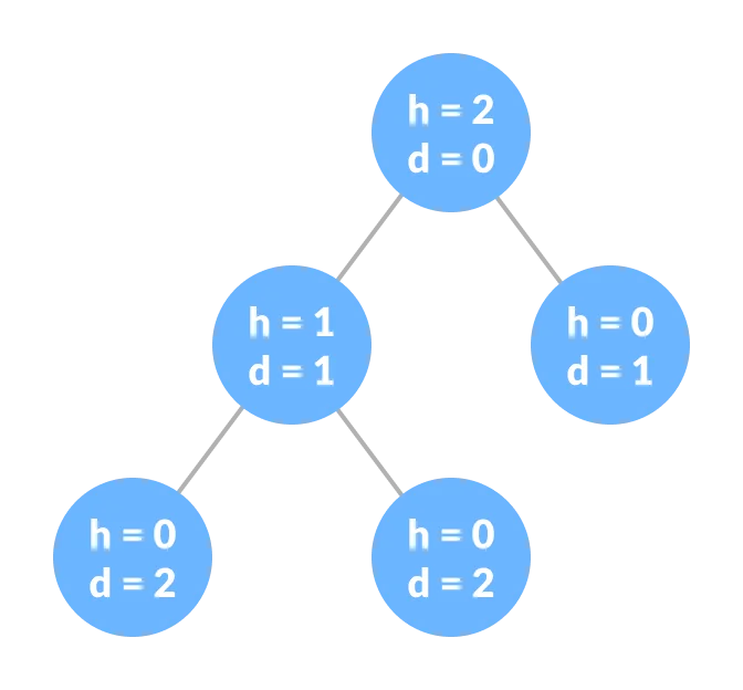
Depth - The depth of a node refers to the total number of edges connecting it to the root node. The total number of edges in the longest path from the root node to the leaf node is the tree's depth. The root node's depth is equal to zero. The terms "level" and "depth" are interchangeable in this context.
Height of node - The number of edges from the node to the deepest leaf determines a node's height (ie. The longest path from the node to a leaf node).
Height of tree - The height of a tree is equal to the depth of the deepest node or the height of the root node.
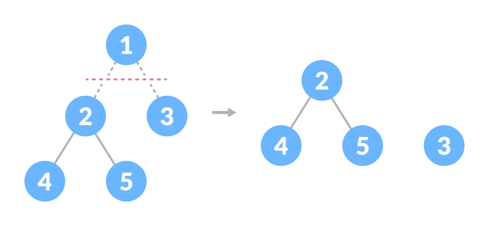
Forest -A forest is a cluster of trees that are not connected in any way.
Key takeaway
A tree is also one of the data structures that represent hierarchical data.
4.2.2 Binary Tree- definition, types (Full/Proper / Plane, Complete, Perfect, Skewed, Balanced)
The Binary tree means that the node can have a maximum of two children. Here, the binary name itself suggests 'two'; therefore, each node can have either 0, 1 or 2 children.
Let's understand the binary tree through an example.
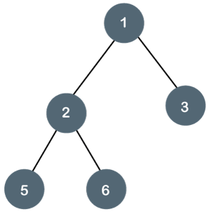
Fig 12: Example
The above tree is a binary tree because each node contains the utmost two children. The logical representation of the above tree is given below:
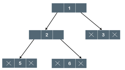
Fig 13: Logical representation
In the above tree, node 1 contains two pointers, i.e., left and a right pointer pointing to the left and right node respectively. The node 2 contains both the nodes (left and right node); therefore, it has two pointers (left and right). The nodes 3, 5 and 6 are the leaf nodes, so all these nodes contain NULL pointer on both left and right parts.
Properties of Binary Tree
● At each level of i, the maximum number of nodes is 2i.
● The height of the tree is defined as the longest path from the root node to the leaf node. The tree which is shown above has a height equal to 3. Therefore, the maximum number of nodes at height 3 is equal to (1+2+4+8) = 15. In general, the maximum number of nodes possible at height h is (20 + 21 + 22+….2h) = 2h+1 -1.
● The minimum number of nodes possible at height h is equal to h+1.
● If the number of nodes is minimum, then the height of the tree would be maximum. Conversely, if the number of nodes is maximum, then the height of the tree would be minimum.
If there are 'n' number of nodes in the binary tree.
The minimum height can be computed as:
As we know that,
n = 2h+1 -1
n+1 = 2h+1
Taking log on both the sides,
Log2(n+1) = log2(2h+1)
Log2(n+1) = h+1
h = log2(n+1) - 1
The maximum height can be computed as:
As we know that,
n = h+1
h= n-1
Types of Binary Tree
There are four types of Binary tree:
● Full/ proper/ strict Binary tree
● Complete Binary tree
● Perfect Binary tree
● Skewed Binary tree
● Balanced Binary tree
Full/ Proper/ Plane
Full binary tree is also called a Strictly binary tree. A strictly binary tree is one in which every non-leaf node in a binary tree has nonempty left and right subtrees. 2n -1 nodes are always present in a strictly binary tree with n leaves.
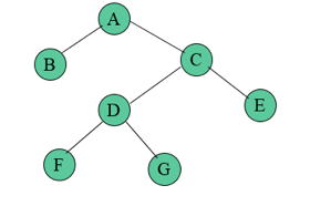
Fig 14: Strict binary tree
A binary tree is said to be strictly binary if every non-leaf node contains nonempty left and right subtrees. To put it another way, in a purely binary tree, all nodes are of degree zero or two, never one.
A binary tree is a finite collection of elements that is either empty or divided into three distinct sections. The first subset has a single element known as the tree's root. The left and right subtrees of the original tree are binary trees, as are the other two subsets. It is possible for a left or right subtree to be empty.
A node of a binary tree is each of the tree's elements, and the tree has nine nodes with A as its root. The left subtree of this tree is rooted at B, whereas the right subtree is rooted at C. The two branches emerging from A to B on the left and to C on the right demonstrate this. An empty subtree is indicated by the lack of a branch.
Complete
The complete binary tree is a tree in which all the nodes are completely filled except the last level. In the last level, all the nodes must be as left as possible. In a complete binary tree, the nodes should be added from the left.
Let's create a complete binary tree.
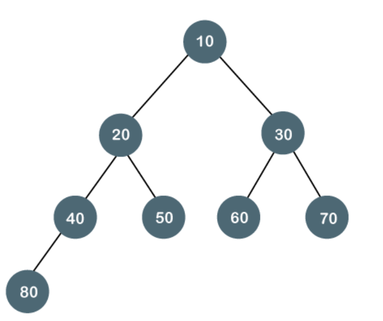
Fig 15: Complete binary tree
The above tree is a complete binary tree because all the nodes are completely filled, and all the nodes in the last level are added at the left first.
Properties of Complete Binary Tree
● The maximum number of nodes in a complete binary tree is 2h+1 - 1.
● The minimum number of nodes in a complete binary tree is 2h.
● The minimum height of a complete binary tree is log2(n+1) - 1.
● The maximum height of a complete binary tree is
Perfect
A perfect binary tree is one in which every internal node has exactly two child nodes and all leaf nodes are at the same level.

Fig 16: Perfect binary tree
A degree of 2 is assigned to all internal nodes.
A perfect binary tree can be defined recursively as:
● It is a perfect binary tree of height h = 0 if a single node has no children. If a node has h > 0,
● it is a perfect binary tree if both of its subtrees are of height h - 1 and are non-overlapping.
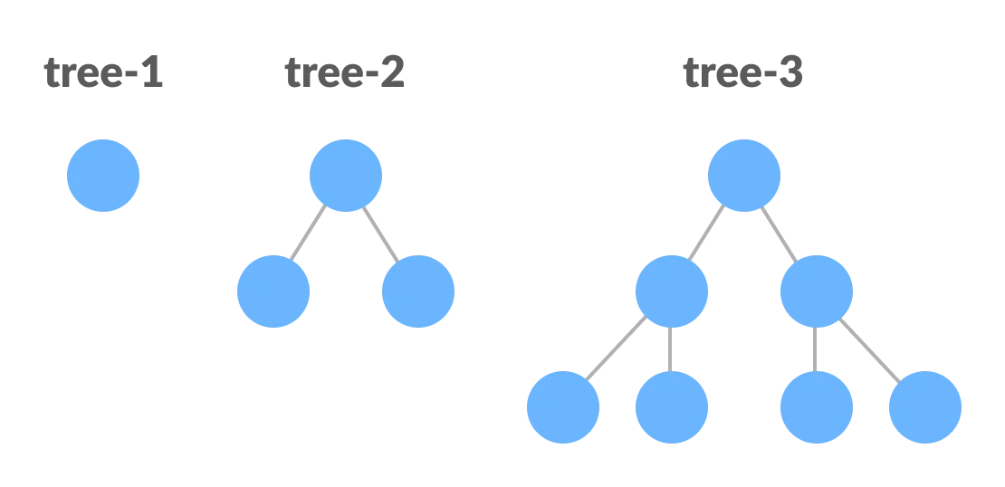
Fig 17: Perfect Binary Tree (Recursive Representation)
Skewed
A skewed binary tree is one that meets both of the following criteria:
● Except for one node, each node has only one child.
● There are no children in the remaining node.
A skewed binary tree is a binary tree with n nodes and a depth of one (n-1).
All except one node in a skewed binary tree has only one child node. There are no children in the remaining node.
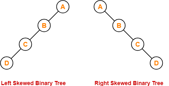
Fig 18: Types of skewed tree
● Left skewed tree - Most nodes in a left-skewed tree have a left child but no corresponding right child.
● Right skewed tree - In a right-skewed tree, the majority of nodes have a right child but no left child.
Balanced
A height balanced binary tree is another name for a balanced binary tree. When the height difference between the left and right subtrees is less than m, where m is usually equal to 1, it is called a binary tree. The number of edges on the longest path between the root node and the leaf node determines a tree's height.
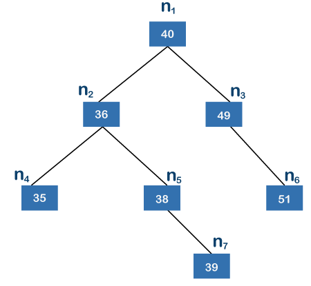
Fig 19: Binary search tree
A binary search tree is one in which each node on the left side has a lower value than its parent node, while the node on the right side has a higher value. The root node in the above tree is n1, while the leaf nodes are n4, n6, and n7. The n7 node is the node that is the furthest away from the root node. There are two edges on the n4 and n6 nodes, and three edges between the root node and the n7 node. The height of the above tree is 3 since n7 is the farthest from the root node.
We'll now see if the tree above is balanced or not. The nodes n2, n4, n5, and n7 are found on the left subtree, while the nodes n3 and n6 are found on the right subtree. Two leaf nodes, n4 and n7, are found in the left subtree. Because there is just one edge connecting nodes n2 and n4 and two between nodes n7 and n2, node n7 is the furthest away from the root node. The left subtree has a height of 2. The right subtree has only one leaf node, n6, and only one edge; thus, the right subtree's height is 1. The difference in height between the left and right subtrees is one.
We may say that the above tree is a height-balanced tree because we received the value 1. This method of computing the height difference should be repeated for each node, such as n2, n3, n4, n5, n6, and n7. We may claim that the above tree is a balanced binary tree because the value of k is not greater than one when we process each node.
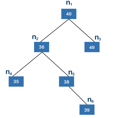
The leaf nodes in the above tree are n6, n4, and n3, with n6 being the farthest node from the root node. Because there are three edges between the root node and the leaf node, the height of the above tree is three. When we take n1 to be the root node, the nodes n2, n4, n5, and n6 are found in the left subtree, whereas the node n3 is found in the right subtree. n2 is a root node in the left subtree, while n4 and n6 are leaf nodes. Because n6 is the farthest node from its root node among the n4 and n6 nodes, and n6 has two edges, the height of the left subtree is 2.
Because there are no children on the left and right sides of the right subtree, its height is 0. Because the left subtree's height is 2 and the right subtree's height is 0, the height difference between the left and right subtrees is 2. The difference in height between the left and right subtrees must not exceed one, according to the definition. The difference in this situation is 2, which is more than 1, making the binary tree above an imbalanced binary search tree.
4.2.3 Binary search tree
A binary search tree is a type of binary tree in which the nodes are organized in a predetermined sequence. This is referred to as an ordered binary tree.
The value of all nodes in the left sub-tree is less than the value of the root in a binary search tree. Similarly, the value of all nodes in the right subtree is larger than or equal to the root's value. This rule will be applied recursively to all of the root's left and right subtrees.
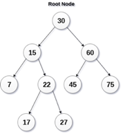
Fig 20: Binary search tree
A Binary Search Tree (BST) is a tree in which all nodes have the properties listed below.
● The key of the left subtree has a lower value than the key of its parent (root) node.
● The value of the right subkey tree's is larger than or equal to the value of the key of its parent (root) node.
● As a result, BST separates all of its sub-trees into two segments: the left and right subtrees, and can be characterized as
Left_subtree (keys) < node (key) ≤ right_subtree (keys)
4.2.4 Operations on BST – Create, Insert, Search, Delete, traversals (Preorder, Inorder, Postorder)
Create
An empty tree with no nodes is built first. The variable/identifier that must point to the root node is set to NULL by default.
Insertion
The insertion operation in a binary search tree takes O(log n) time to complete. A new node is always added as a leaf node in a binary search tree. The following is how the insertion procedure is carried out...
Step 1: Create a newNode with the specified value and NULL left and right.
Step 2: Make sure the tree isn't empty.
Step 3 - Set root to newNode if the tree is empty.
Step 4 - If the tree isn't empty, see if newNode's value is smaller or larger than the node's value (here it is root node).
Step 5 - Go to the node's left child if newNode is smaller or equal to it. Move to new Nodes right child if the newNode is larger than the node.
Step 6- Continue in this manner until we reach the leaf node (i.e., reaches to NULL).
Step 7 - Once you've reached the leaf node, insert the newNode as a left child if it's smaller or equal to the leaf node, or as a right child otherwise.
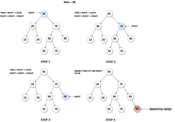
Fig 21: Example of insertion
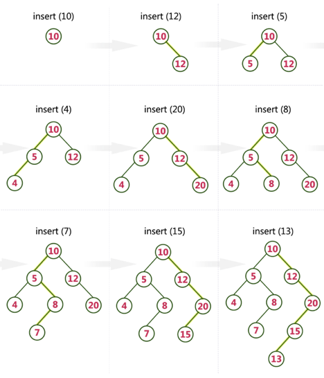
Example
Create a Binary Search Tree by adding the integers in the following order…
10,12,5,4,20,8,7,15 and 13
The following items are added into a Binary Search Tree in the following order...
Searching
The search operation in a binary search tree takes O(log n) time to complete. The following is how the search is carried out...
Step 1: Ask the user for the search element.
Step 2: Compare the value of the root node in the tree to the search element.
Step 3 - If both match, the function will display "Given node is found!!!" and the function will be terminated.
Step 4 - If neither of the search elements match, see if the search element is smaller or larger than the node value.
Step 5 - Continue searching in the left subtree if the search element is smaller.
Step 6- If the search element is larger, move on to the correct subtree and continue the search.
Step 7 - Continue in this manner until the exact element is found or the search element is compared to the leaf node.
Step 8 - If we reach a node with a value equal to the search value, we'll get "Element found" and the function will end.
Step 9 - If we get to the leaf node and it doesn't match the search element, we'll see "Element not found" and the function will end.
Algorithm to search an element in Binary search tree
Search (root, item)
Step 1 - if (item = root → data) or (root = NULL)
Return root
Else if (item < root → data)
Return Search(root → left, item)
Else
Return Search(root → right, item)
END if
Step 2 - END
Deletion
The deletion process in a binary search tree takes O(log n) time to complete. The three scenarios for removing a node from a Binary search tree are as follows...
Case 1: Deleting a Leaf node (A node with no children)
Case 2: Deleting a node with one child
Case 3: Deleting a node with two children
Case 1: Deleting a Leaf node
To delete a leaf node from BST, follow these steps...
Step 1: Using the search function, locate the node to be eliminated.
Step 2 - If the node is a leaf, delete it with the free function and end the function.
Case 2: Deleting a node with one child
To delete a node with one child from BST, we utilize the procedures below...
Step 1: Using the search function, locate the node to be eliminated.
Step 2 - Create a link between the parent node and the child node if it only has one child.
Step 3: Using the free function, delete the node and exit the function
Case 3: Deleting a node with two children
To delete a node with two children from BST, we utilize the procedures below...
Step 1: Using the search function, locate the node to be eliminated.
Step 2 - Find the largest node in the left subtree (OR the smallest node in the right subtree) if it has two children.
Step 3 - Swap the deleting node with the node discovered in the previous step.
Step 4 - Next, see if deleting the node resulted in case 1 or case 2, if not, move to step 2.
Step 5 - If case 1 applies, delete it using case 1 reasoning.
Step 6- If case 2 applies, delete it using case 2 reasoning.
Step 7 - Continue in this manner until the node has been removed from the tree.
Traversals
Traversal is a process to visit all the nodes of a tree and may print their values too. Because all nodes are connected via edges (links) we always start from the root (head) node. That is, we cannot randomly access a node in a tree. There are three ways which we use to traverse a tree −
● In-order Traversal
● Pre-order Traversal
● Post-order Traversal
Generally, we traverse a tree to search or locate a given item or key in the tree or to print all the values it contains.
In-order Traversal
In this traversal method, the left subtree is visited first, then the root and later the right subtree. We should always remember that every node may represent a subtree itself.
If a binary tree is traversed in-order, the output will produce sorted key values in an ascending order.

Fig 22: Inorder
We start from A, and following in-order traversal, we move to its left subtree B. B is also traversed in-order. The process goes on until all the nodes are visited. The output of inorder traversal of this tree will be −
D → B → E → A → F → C → G
Algorithm
Until all nodes are traversed −
Step 1 − Recursively traverse left subtree.
Step 2 − Visit root node.
Step 3 − Recursively traverse right subtree.
Pre-order Traversal
In this traversal method, the root node is visited first, then the left subtree and finally the right subtree.

Fig 23: Pre order
We start from A, and following pre-order traversal, we first visit A itself and then move to its left subtree B. B is also traversed pre-order. The process goes on until all the nodes are visited. The output of pre-order traversal of this tree will be −
A → B → D → E → C → F → G
Algorithm
Until all nodes are traversed −
Step 1 − Visit root node.
Step 2 − Recursively traverse left subtree.
Step 3 − Recursively traverse right subtree.
Post-order Traversal
In this traversal method, the root node is visited last, hence the name. First we traverse the left subtree, then the right subtree and finally the root node.

Fig 24: Post order
We start from A, and following Post-order traversal, we first visit the left subtree B. B is also traversed post-order. The process goes on until all the nodes are visited. The output of post-order traversal of this tree will be −
D → E → B → F → G → C → A
Algorithm
Until all nodes are traversed −
Step 1 − Recursively traverse left subtree.
Step 2 − Recursively traverse the right subtree.
Step 3 − Visit the root node.
References:
- Data structure through C++- Yashwant Kanitkar (BPB Publications)
- Principles of Data structures using c++ - Vinu V. Das(New Age International Publication)
- Data Structures with C- SEYMOUR LIPSCHUTZ( Tata McGraw-Hill)
- Data structures, Algorithms and Applications in C++, S.Sahni, University Press (India) Pvt.Ltd, 2nd edition, Universities Press Orient Longman Pvt. Ltd.
- Https://www.gatevidyalay.com/tree-data-structure-tree-terminology/
- Https://www.programiz.com/dsa/trees