UNIT-1
Introduction & Overview
Data Structure can be defined as the group of data elements which provides an efficient way of storing and organising data in the computer so that it can be used efficiently. Some examples of Data Structures are arrays, Linked List, Stack, Queue, etc. Data Structures are widely used in almost every aspect of Computer Science i.e. Operating System, Compiler Design, Artifical intelligence, Graphics and many more.
Data Structures are the main part of many computer science algorithms as they enable the programmers to handle the data in an efficient way. It plays a vitle role in enhancing the performance of a software or a program as the main function of the software is to store and retrieve the user's data as fast as possible
Data structures are the building blocks of any program or the software. Choosing the appropriate data structure for a program is the most difficult task for a programmer. Following terminology is used as far as data structures are concerned
Data: Data can be defined as an elementary value or the collection of values, for example, student's name and its id are the data about the student.
Group Items: Data items which have subordinate data items are called Group item, for example, name of a student can have first name and the last name.
Record: Record can be defined as the collection of various data items, for example, if we talk about the student entity, then its name, address, course and marks can be grouped together to form the record for the student.
File: A File is a collection of various records of one type of entity, for example, if there are 60 employees in the class, then there will be 20 records in the related file where each record contains the data about each employee.
Attribute and Entity: An entity represents the class of certain objects. it contains various attributes. Each attribute represents the particular property of that entity.
Field: Field is a single elementary unit of information representing the attribute of an entity.
As applications are getting complexed and amount of data is increasing day by day, there may arrise the following problems:
Processor speed: To handle very large amout of data, high speed processing is required, but as the data is growing day by day to the billions of files per entity, processor may fail to deal with that much amount of data.
Data Search: Consider an inventory size of 106 items in a store, If our application needs to search for a particular item, it needs to traverse 106 items every time, results in slowing down the search process.
Multiple requests: If thousands of users are searching the data simultaneously on a web server, then there are the chances that a very large server can be failed during that process
in order to solve the above problems, data structures are used. Data is organized to form a data structure in such a way that all items are not required to be searched and required data can be searched instantly.
Efficiency: Efficiency of a program depends upon the choice of data structures. For example: suppose, we have some data and we need to perform the search for a perticular record. In that case, if we organize our data in an array, we will have to search sequentially element by element. hence, using array may not be very efficient here. There are better data structures which can make the search process efficient like ordered array, binary search tree or hash tables.
Reusability: Data structures are reusable, i.e. once we have implemented a particular data structure, we can use it at any other place. Implementation of data structures can be compiled into libraries which can be used by different clients.
Abstraction: Data structure is specified by the ADT which provides a level of abstraction. The client program uses the data structure through interface only, without getting into the implementation details.
|
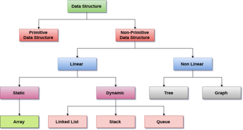
Fig 1 – Classification of data structure
Linear Data Structures: A data structure is called linear if all of its elements are arranged in the linear order. In linear data structures, the elements are stored in non-hierarchical way where each element has the successors and predecessors except the first and last element.
Types of Linear Data Structures are given below:
Arrays: An array is a collection of similar type of data items and each data item is called an element of the array. The data type of the element may be any valid data type like char, int, float or double.
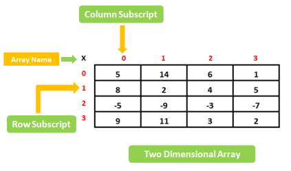
The elements of array share the same variable name but each one carries a different index number known as subscript. The array can be one dimensional, two dimensional or multidimensional.
The individual elements of the array age are:
age[0], age[1], age[2], age[3],......... age[98], age[99].
Linked List: Linked list is a linear data structure which is used to maintain a list in the memory. It can be seen as the collection of nodes stored at non-contiguous memory locations. Each node of the list contains a pointer to its adjacent node.
Stack: Stack is a linear list in which insertion and deletions are allowed only at one end, called top.
A stack is an abstract data type (ADT), can be implemented in most of the programming languages. It is named as stack because it behaves like a real-world stack, for example: - piles of plates or deck of cards etc.
Queue: Queue is a linear list in which elements can be inserted only at one end called rear and deleted only at the other end called front.
It is an abstract data structure, similar to stack. Queue is opened at both end therefore it follows First-In-First-Out (FIFO) methodology for storing the data items.
Non Linear Data Structures: This data structure does not form a sequence i.e. each item or element is connected with two or more other items in a non-linear arrangement. The data elements are not arranged in sequential structure.
Types of Non-Linear Data Structures are given below:
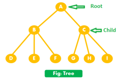
Trees: Trees are multilevel data structures with a hierarchical relationship among its elements known as nodes. The bottommost nodes in the herierchy are called leaf node while the topmost node is called root node. Each node contains pointers to point adjacent nodes.
Tree data structure is based on the parent-child relationship among the nodes. Each node in the tree can have more than one children except the leaf nodes whereas each node can have atmost one parent except the root node. Trees can be classfied into many categories which will be discussed later in this tutorial.
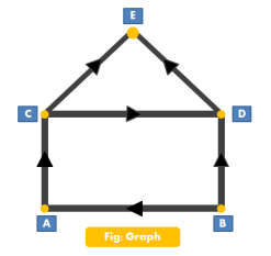
Graphs: Graphs can be defined as the pictorial representation of the set of elements (represented by vertices) connected by the links known as edges. A graph is different from tree in the sense that a graph can have cycle while the tree can not have the one.
1) Traversing: Every data structure contains the set of data elements. Traversing the data structure means visiting each element of the data structure in order to perform some specific operation like searching or sorting.
Example: If we need to calculate the average of the marks obtained by a student in 6 different subject, we need to traverse the complete array of marks and calculate the total sum, then we will devide that sum by the number of subjects i.e. 6, in order to find the average.
2) Insertion: Insertion can be defined as the process of adding the elements to the data structure at any location.
If the size of data structure is n then we can only insert n-1 data elements into it.
3) Deletion:The process of removing an element from the data structure is called Deletion. We can delete an element from the data structure at any random location.
If we try to delete an element from an empty data structure then underflow occurs.
4) Searching: The process of finding the location of an element within the data structure is called Searching. There are two algorithms to perform searching, Linear Search and Binary Search. We will discuss each one of them later in this tutorial.
5) Sorting: The process of arranging the data structure in a specific order is known as Sorting. There are many algorithms that can be used to perform sorting, for example, insertion sort, selection sort, bubble sort, etc.
6) Merging: When two lists List A and List B of size M and N respectively, of similar type of elements, clubbed or joined to produce the third list, List C of size (M+N), then this process is called merging
Key takeaway
Data Structure can be defined as the group of data elements which provides an efficient way of storing and organising data in the computer so that it can be used efficiently. Some examples of Data Structures are arrays, Linked List, Stack, Queue, etc. Data Structures are widely used in almost every aspect of Computer Science i.e. Operating System, Compiler Design, Artifical intelligence, Graphics and many more.
Data Structures are the main part of many computer science algorithms as they enable the programmers to handle the data in an efficient way. It plays a vitle role in enhancing the performance of a software or a program as the main function of the software is to store and retrieve the user's data as fast as possible
As we know that programming entirely revolves around data. It is data over which all the business logic gets implemented and it’s the flow of data which comprises the functionality of an application or project. So it becomes very much important to organize and store the data for its optimized use and does the effective programming with good data model.
In general both data type and data structure seems to be the same thing as both deals with the nature and organizing of data but among two one describes the type and nature of data while other represents the collections in which that data can be stored.
Following are the important differences between Data Type and Data Structure
Sr. No. | Key | Data Type | Data Structure |
1 | Definition | Data type is the representation of nature and type of data that has been going to be used in programming or in other words data type describes all that data which share a common property. For example an integer data type describes every integer that the computers can handle. | On other hand Data structure is the collection that holds data which can be manipulated and used in programming so that operations and algorithms can be more easily applied. For example tree type data structures often allow for efficient searching algorithms. |
2 | Implementation | Data type in programming are implemented in abstract implementation whose definition is provided by different languages in different ways. | On other hand Data type in programming are implemented in concrete implementation as their definition is already defined by the language that what type of data they going to store and deal with. |
3 | Storage | In case of data type the value of data is not stored as it only represents the type of data that can be get stored. | On other hand data structure holds the data along with its value that actually acquires the space in main memory of the computer. Also data structure can hold different kind and types of data within one single object |
4 | Assignment | As data type already represents the type of value that can be stored so values can directly be assigned to the data type variables. | On other hand in case of data structure the data is assigned to using some set of algorithms and operations like push, pop and so on. |
5 | Performance | If case of data type only type and nature of data is concern so there in no issue of time complexity. | On other hand time complexity comes in case of data structure as it mainly deals with manipulation and execution of logic over data that it stored. |
Key takeaway
As we know that programming entirely revolves around data. It is data over which all the business logic gets implemented and it’s the flow of data which comprises the functionality of an application or project. So it becomes very much important to organize and store the data for its optimized use and does the effective programming with good data model.
In general both data type and data structure seems to be the same thing as both deals with the nature and organizing of data but among two one describes the type and nature of data while other represents the collections in which that data can be stored.
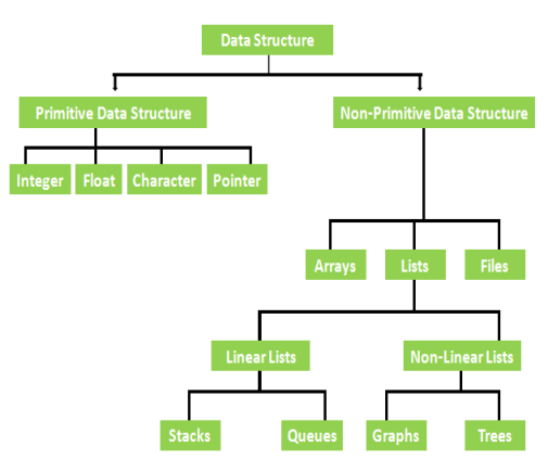
Classification of Data Structure, Data Structures are normally divided into two broad categories:
(1) Primitive Data Structures
(2) Non-Primitive Data Structures
|
Fig 2 – Data structure classification
What is Primitive Data Structures?
These are basic structures and are directly operated upon by the machine instructions.
These to general have different representations on different computers, Integer, Floating point numbers, character-constants, string constants, pointers, etc.
Example of Primitive Data Structures with explanation
- Float
- Integer
- Character
- Pointer
What is Float?
Float: When you listen to float in the data structure, the first thing which comes in mind, what is mean of float? if you don’t know, let’s explain me, Float is a tern in a data structure which is used in the various programming language, for defining the variable with a fractional value.
this is the contrast of the integer data type, therefore, the numbers created using of float variable declaration will have decimal point, which means have to digit on both sides of a decimal point. In other words, we can say that programmers used float term before the name of a variable.
as a result, declare a value for the float variable by using the name of variables, after that adding the equal sign, and follows as according to the value.
What is an Integer?
An integer defined as a whole number, not a fraction number, the integer number can be positive, negative or zero number. such as 10, 11, 0, -7, -67 and 5148 are all integers. integer number can’t have decimal places.
therefore, when two integer numbers are added, subtracted or multiplied, the result always comes as an integer.
What is Character?
Character in the data structure represents letter and symbol such as a, B, f, R, “.” , “-” and whitespace. therefore, it can store the basic character set. it can hold one letter/symbol like n, F,d, etc. characters can also be of different types.
What is Pointer?
A pointer represents a storage location in memory (RAM).in the RAM contains many cells and the values are stored in these cells. each cell in memory is 1 byte and the memory address is always an unsigned integer, therefore, each cell has a unique address to identify it.
What is Non-Primitive Data Structures?
Generally, language provides a way of defining our own data type. such data types are kept under the non-primitive data structure category.
therefore, these are the more sophisticated data structure. These are derived from the primitive data structure.
The non-primitive data structures emphasize the structuring of a group of homogeneous or heterogeneous data items.
therefore, Arrays, lists, and files are the example.
consequently, we can define, the design of an efficient data structure must take operations to be performed on the data structure into account.
furthermore, let’s see the example, consider a data structure consisting of a set of data items.
The data structure is to be manipulated to a number of major program functions.
finally, when evaluating the operations to be performed on the data structure here, an abstract data type is defined to use it in subsequent programs.
Example of Primitive Data Structures with explanation
- Arrays
- Lists
- Files
- Stacks
- Queues
- Graphs
- trees
What is Arrays?
An array is defined as it is a collection of items stored at contiguous memory locations. we can also say that arrays are the set of homogeneous data elements stored in RAM, therefore, it can hold only one type of data.
Therefore, the data may be all floating numbers or all characters or all integers numbers. therefore, array makes it easier to calculate, what is the position of each element by simply adding an offset to a base value.
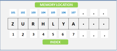
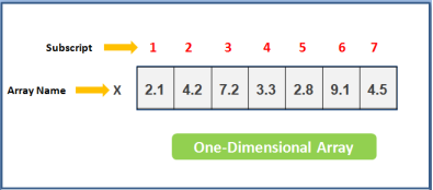
Therefore, Single sub-scripted values are called linear array or one-dimensional array and two-subscripted variables are called as two-dimensional array.let’s understand better as given below diagram.
|
Fig 3 – Memory location
|
Fig 4 – one dimensional array
|
Fig 5 – Two dimensional array
What are Lists?
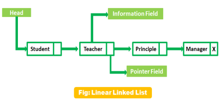
A Lists is defined as it is a collection pf a variable number of data items. lists or sequence is an abstract data type, which always represents a countable number of ordered values, Every list element contains at least two fields, one field is used for storing the data and another filed is used for storing the address of the next element.
therefore we can say that lists are an example of containers. as they contain other values. if the same value occurs multiple times, then each occurrence is considered a distinct item.
Diagram:
|
Fig 6 – Linear linked list
What is Files?
Files contain information, and this information stored permanently in the Hard Disk and Floppy Disk, this disk also knows as a secondary storage device. you can store a little byte of data and a large amount of data in secondary devices.
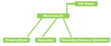
therefore, A file name always contains the primary and secondary name and dot(.) is used for separating. for understanding in a better way see the below Diagram
|
Fig 7 – File name
What is Stacks?
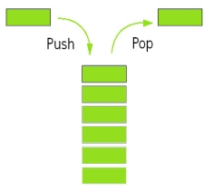
A stack is a basic data structure, it’s defined as an ordered collection of elements represented by a real physical stack or pile. liner data structure features insertion and deletion of items take place at one end called top of the stack.
Therefore, In these structure data set as a stack of books or plates, in the stack, you can remove the item from the top order. you can use these concepts or structures all throughout programming. the implementation of the stack also know as LIFO (Last in First Out)
these are the three basic concepts that can be performed on stacks.
1) push (insert the items into a stack)
2) Pop (delete an item from the stack)
3) Pip (displaying the content of the stack)
Diagram:
|
Fig 8 – Stack
What are Queues?
Queue defined (FIFO) First In First Out type of data structure. Queues are also the part of non-primitive linear data structure, therefore in Queues process, we can insert an element in a queue from the REAR end and delete an element from the FRONT end only.
Therefore, Implement queues with using two ways:
- Pointers
- Arrays
|
Fig 9 - Queue
What are the Graphs?
There are different types of graphs :
- Connected Graph
- Non-Connected Graph
- Directed Graph
- Non-Directed Graph
therefore, graphs are the non-linear and non-primitive type of data structure. graph is representing the different types of physical design structures such as used in Chemistry, physics, maths & Engineering Science.
|
Fig 10 - Graph
What are the trees?
In the classification of data structure, Trees also come in the non-primitive and non-linear category data structure, using tree we can represent a hierarchical relationship between the data elements.
|
Fig 11 - Tree
Data Structure the most commonly used operations
As a result, in the Classification of Data Structure, Data Structure the most commonly used operations are broadly categorized into four types:
(1) Create
(2) Delete
(3) Selection
(4) Update
The CREATE operation (it can be defined) results in reserving memory for the program elements.
This can be done by a declaration statement.
The creation of data structure may take place either during compile -time or during Runtime.
therefore, on the other hand, DELETE operation destroys the memory space allocated for the specified data structure Malloc() and free ()
as a result, the function of C language is used for these two operations respectively.
The SELECTION operation can be defined as its deals with accessing particular data within a data structure.
And the last operations UPDATE, as the name implies, it updates or modifies the data in the data structure.Hence, in the Classification of Data Structure the operation Probably new data may be entered or previously stored data may be deleted.
so, in Classification of Data Structure, Other operations performed on data structure include:
(1) Searching
(2) Sorting
(3) Merging
Searching operation finds the presence of the desired data item in the list of the data item.
it can define that Sorting is the process of arranging all data items in a data structure in a particular order say for example, either in ascending order or in descending order.
furthermore, finally MERGING is a process of combining the data items of two different sorted lists into a single sorted list.
Key takeaway
These are basic structures and are directly operated upon by the machine instructions.
These to general have different representations on different computers, Integer, Floating point numbers, character-constants, string constants, pointers, etc.
An algorithm is a process or a set of rules required to perform calculations or some other problem-solving operations especially by a computer. The formal definition of an algorithm is that it contains the finite set of instructions which are being carried in a specific order to perform the specific task. It is not the complete program or code; it is just a solution (logic) of a problem, which can be represented either as an informal description using a Flowchart or Pseudocode.
Characteristics of an Algorithm
The following are the characteristics of an algorithm:
- Input: An algorithm has some input values. We can pass 0 or some input value to an algorithm.
- Output: We will get 1 or more output at the end of an algorithm.
- Unambiguity: An algorithm should be unambiguous which means that the instructions in an algorithm should be clear and simple.
- Finiteness: An algorithm should have finiteness. Here, finiteness means that the algorithm should contain a limited number of instructions, i.e., the instructions should be countable.
- Effectiveness: An algorithm should be effective as each instruction in an algorithm affects the overall process.
- Language independent: An algorithm must be language-independent so that the instructions in an algorithm can be implemented in any of the languages with the same output.
- Problem: A problem can be a real-world problem or any instance from the real-world problem for which we need to create a program or the set of instructions. The set of instructions is known as an algorithm.
- Algorithm: An algorithm will be designed for a problem which is a step by step procedure.
- Input: After designing an algorithm, the required and the desired inputs are provided to the algorithm.
- Processing unit: The input will be given to the processing unit, and the processing unit will produce the desired output.
- Output: The output is the outcome or the result of the program.
We need algorithms because of the following reasons:
- Scalability: It helps us to understand the scalability. When we have a big real-world problem, we need to scale it down into small-small steps to easily analyze the problem.
- Performance: The real-world is not easily broken down into smaller steps. If the problem can be easily broken into smaller steps means that the problem is feasible.
Let's understand the algorithm through a real-world example. Suppose we want to make a lemon juice, so following are the steps required to make a lemon juice:
Step 1: First, we will cut the lemon into half.
Step 2: Squeeze the lemon as much you can and take out its juice in a container.
Step 3: Add two tablespoon sugar in it.
Step 4: Stir the container until the sugar gets dissolved.
Step 5: When sugar gets dissolved, add some water and ice in it.
Step 6: Store the juice in a fridge for 5 to minutes.
Step 7: Now, it's ready to drink.
The above real-world can be directly compared to the definition of the algorithm. We cannot perform the step 3 before the step 2, we need to follow the specific order to make lemon juice. An algorithm also says that each and every instruction should be followed in a specific order to perform a specific task.
Now we will look an example of an algorithm in programming.
We will write an algorithm to add two numbers entered by the user.
The following are the steps required to add two numbers entered by the user:
Step 1: Start
Step 2: Declare three variables a, b, and sum.
Step 3: Enter the values of a and b.
Step 4: Add the values of a and b and store the result in the sum variable, i.e., sum=a+b.
Step 5: Print sum
Step 6: Stop
The following are the factors that we need to consider for designing an algorithm:
- Modularity: If any problem is given and we can break that problem into small-small modules or small-small steps, which is a basic definition of an algorithm, it means that this feature has been perfectly designed for the algorithm.
- Correctness: The correctness of an algorithm is defined as when the given inputs produce the desired output, which means that the algorithm has been designed algorithm. The analysis of an algorithm has been done correctly.
- Maintainability: Here, maintainability means that the algorithm should be designed in a very simple structured way so that when we redefine the algorithm, no major change will be done in the algorithm.
- Functionality: It considers various logical steps to solve the real-world problem.
- Robustness: Robustness means that how an algorithm can clearly define our problem.
- User-friendly: If the algorithm is not user-friendly, then the designer will not be able to explain it to the programmer.
- Simplicity: If the algorithm is simple then it is easy to understand.
- Extensibility: If any other algorithm designer or programmer wants to use your algorithm then it should be extensible.
- Theoretical importance: When any real-world problem is given to us and we break the problem into small-small modules. To break down the problem, we should know all the theoretical aspects.
- Practical importance: As we know that theory cannot be completed without the practical implementation. So, the importance of algorithm can be considered as both theoretical and practical.
The following are the issues that come while designing an algorithm:
- How to design algorithms: As we know that an algorithm is a step-by-step procedure so we must follow some steps to design an algorithm.
- How to analyze algorithm efficiency
The following are the approaches used after considering both the theoretical and practical importance of designing an algorithm:
- Brute force algorithm: The general logic structure is applied to design an algorithm. It is also known as an exhaustive search algorithm that searches all the possibilities to provide the required solution. Such algorithms are of two types:
- Optimizing: Finding all the solutions of a problem and then take out the best solution or if the value of the best solution is known then it will terminate if the best solution is known.
- Sacrificing: As soon as the best solution is found, then it will stop.
- Divide and conquer: It is a very implementation of an algorithm. It allows you to design an algorithm in a step-by-step variation. It breaks down the algorithm to solve the problem in different methods. It allows you to break down the problem into different methods, and valid output is produced for the valid input. This valid output is passed to some other function.
- Greedy algorithm: It is an algorithm paradigm that makes an optimal choice on each iteration with the hope of getting the best solution. It is easy to implement and has a faster execution time. But, there are very rare cases in which it provides the optimal solution.
- Dynamic programming: It makes the algorithm more efficient by storing the intermediate results. It follows five different steps to find the optimal solution for the problem:
- It breaks down the problem into a subproblem to find the optimal solution.
- After breaking down the problem, it finds the optimal solution out of these subproblems.
- Stores the result of the subproblems is known as memorization.
- Reuse the result so that it cannot be recomputed for the same subproblems.
- Finally, it computes the result of the complex program.
- Branch and Bound Algorithm: The branch and bound algorithm can be applied to only integer programming problems. This approach divides all the sets of feasible solutions into smaller subsets. These subsets are further evaluated to find the best solution.
- Randomized Algorithm: As we have seen in a regular algorithm, we have predefined input and required output. Those algorithms that have some defined set of inputs and required output, and follow some described steps are known as deterministic algorithms. What happens that when the random variable is introduced in the randomized algorithm?. In a randomized algorithm, some random bits are introduced by the algorithm and added in the input to produce the output, which is random in nature. Randomized algorithms are simpler and efficient than the deterministic algorithm.
- Backtracking: Backtracking is an algorithmic technique that solves the problem recursively and removes the solution if it does not satisfy the constraints of a problem.
The major categories of algorithms are given below:
- Sort: Algorithm developed for sorting the items in a certain order.
- Search: Algorithm developed for searching the items inside a data structure.
- Delete: Algorithm developed for deleting the existing element from the data structure.
- Insert: Algorithm developed for inserting an item inside a data structure.
- Update: Algorithm developed for updating the existing element inside a data structure.
The algorithm can be analyzed in two levels, i.e., first is before creating the algorithm, and second is after creating the algorithm. The following are the two analysis of an algorithm:
- Priori Analysis: Here, priori analysis is the theoretical analysis of an algorithm which is done before implementing the algorithm. Various factors can be considered before implementing the algorithm like processor speed, which has no effect on the implementation part.
- Posterior Analysis: Here, posterior analysis is a practical analysis of an algorithm. The practical analysis is achieved by implementing the algorithm using any programming language. This analysis basically evaluate that how much running time and space taken by the algorithm.
The performance of the algorithm can be measured in two factors:
- Time complexity: The time complexity of an algorithm is the amount of time required to complete the execution. The time complexity of an algorithm is denoted by the big O notation. Here, big O notation is the asymptotic notation to represent the time complexity. The time complexity is mainly calculated by counting the number of steps to finish the execution. Let's understand the time complexity through an example.
- sum=0;
- // Suppose we have to calculate the sum of n numbers.
- for i=1 to n
- sum=sum+i;
- // when the loop ends then sum holds the sum of the n numbers
- return sum;
In the above code, the time complexity of the loop statement will be atleast n, and if the value of n increases, then the time complexity also increases. While the complexity of the code, i.e., return sum will be constant as its value is not dependent on the value of n and will provide the result in one step only. We generally consider the worst-time complexity as it is the maximum time taken for any given input size.
- Space complexity: An algorithm's space complexity is the amount of space required to solve a problem and produce an output. Similar to the time complexity, space complexity is also expressed in big O notation.
For an algorithm, the space is required for the following purposes:
- To store program instructions
- To store constant values
- To store variable values
- To track the function calls, jumping statements, etc.
Auxiliary space: The extra space required by the algorithm, excluding the input size, is known as an auxiliary space. The space complexity considers both the spaces, i.e., auxiliary space, and space used by the input.
So,
Space complexity = Auxiliary space + Input size.
The following are the types of algorithm:
- Search Algorithm
- Sort Algorithm
Search Algorithm
On each day, we search for something in our day to day life. Similarly, with the case of computer, huge data is stored in a computer that whenever the user asks for any data then the computer searches for that data in the memory and provides that data to the user. There are mainly two techniques available to search the data in an array:
- Linear search
- Binary search
Linear Search
Linear search is a very simple algorithm that starts searching for an element or a value from the beginning of an array until the required element is not found. It compares the element to be searched with all the elements in an array, if the match is found, then it returns the index of the element else it returns -1. This algorithm can be implemented on the unsorted list.
Binary Search
A Binary algorithm is the simplest algorithm that searches the element very quickly. It is used to search the element from the sorted list. The elements must be stored in sequential order or the sorted manner to implement the binary algorithm. Binary search cannot be implemented if the elements are stored in a random manner. It is used to find the middle element of the list.
Sorting algorithms are used to rearrange the elements in an array or a given data structure either in an ascending or descending order. The comparison operator decides the new order of the elements.
Why do we need a sorting algorithm?
- An efficient sorting algorithm is required for optimizing the efficiency of other algorithms like binary search algorithm as a binary search algorithm requires an array to be sorted in a particular order, mainly in ascending order.
- It produces information in a sorted order, which is a human-readable format.
- Searching a particular element in a sorted list is faster than the unsorted list.
Key takeaway
An algorithm is a process or a set of rules required to perform calculations or some other problem-solving operations especially by a computer. The formal definition of an algorithm is that it contains the finite set of instructions which are being carried in a specific order to perform the specific task. It is not the complete program or code; it is just a solution (logic) of a problem, which can be represented either as an informal description using a Flowchart or Pseudocode.
Reference:
1 Data structure & algorithm analysis in C by Mark Allen Weiss published by Pearson Education (LPE)
2 Introduction to Data structure in C by A.N. Kathie published by Pearson Education (LPE)
