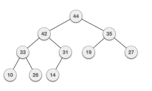
UNIT-5
Trees
The Binary tree means that the node can have maximum two children. Here, binary name itself suggests that 'two'; therefore, each node can have either 0, 1 or 2 children.
Let's understand the binary tree through an example.
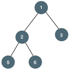
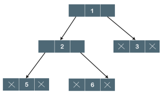
Fig1 - Example The above tree is a binary tree because each node contains the utmost two children. The logical representation of the above tree is given below:
Fig 2 - logical representation |
In the above tree, node 1 contains two pointers, i.e., left and a right pointer pointing to the left and right node respectively. The node 2 contains both the nodes (left and right node); therefore, it has two pointers (left and right). The nodes 3, 5 and 6 are the leaf nodes, so all these nodes contain NULL pointer on both left and right parts.
- At each level of i, the maximum number of nodes is 2i.
- The height of the tree is defined as the longest path from the root node to the leaf node. The tree which is shown above has a height equal to 3. Therefore, the maximum number of nodes at height 3 is equal to (1+2+4+8) = 15. In general, the maximum number of nodes possible at height h is (20 + 21 + 22+….2h) = 2h+1 -1.
- The minimum number of nodes possible at height h is equal to h+1.
- If the number of nodes is minimum, then the height of the tree would be maximum. Conversely, if the number of nodes is maximum, then the height of the tree would be minimum.
If there are 'n' number of nodes in the binary tree.
The minimum height can be computed as:
As we know that,
n = 2h+1 -1
n+1 = 2h+1
Taking log on both the sides,
log2(n+1) = log2(2h+1)
log2(n+1) = h+1
h = log2(n+1) - 1
The maximum height can be computed as:
As we know that,
n = h+1
h= n-1
There are four types of Binary tree:
- Full/ proper/ strict Binary tree
- Complete Binary tree
- Perfect Binary tree
- Degenerate Binary tree
- Balanced Binary tree
1. Full/ proper/ strict Binary tree
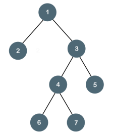
The full binary tree is also known as a strict binary tree. The tree can only be considered as the full binary tree if each node must contain either 0 or 2 children. The full binary tree can also be defined as the tree in which each node must contain 2 children except the leaf nodes.
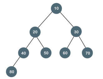
Let's look at the simple example of the Full Binary tree.
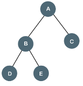
Fig 3 - Example
In the above tree, we can observe that each node is either containing zero or two children; therefore, it is a Full Binary tree.
Properties of Full Binary Tree
- The number of leaf nodes is equal to the number of internal nodes plus 1. In the above example, the number of internal nodes is 5; therefore, the number of leaf nodes is equal to 6.
- The maximum number of nodes is the same as the number of nodes in the binary tree, i.e., 2h+1 -1.
- The minimum number of nodes in the full binary tree is 2*h-1.
- The minimum height of the full binary tree is log2(n+1) - 1.
- The maximum height of the full binary tree can be computed as:
n= 2*h - 1
n+1 = 2*h
h = n+1/2
Complete Binary Tree
The complete binary tree is a tree in which all the nodes are completely filled except the last level. In the last level, all the nodes must be as left as possible. In a complete binary tree, the nodes should be added from the left.
Let's create a complete binary tree.
|
Fig 4 - Complete binary tree
The above tree is a complete binary tree because all the nodes are completely filled, and all the nodes in the last level are added at the left first.
Properties of Complete Binary Tree
- The maximum number of nodes in complete binary tree is 2h+1 - 1.
- The minimum number of nodes in complete binary tree is 2h.
- The minimum height of a complete binary tree is log2(n+1) - 1.
- The maximum height of a complete binary tree is
Perfect Binary Tree
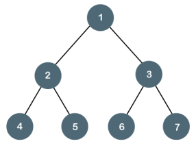
A tree is a perfect binary tree if all the internal nodes have 2 children, and all the leaf nodes are at the same level.
|
Fig 5 - Perfect Binary Tree
Let's look at a simple example of a perfect binary tree.
The below tree is not a perfect binary tree because all the leaf nodes are not at the same level.
|
Fig 6 - Example
Note: All the perfect binary trees are the complete binary trees as well as the full binary tree, but vice versa is not true, i.e., all complete binary trees and full binary trees are the perfect binary trees.
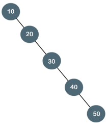
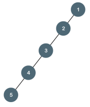
The degenerate binary tree is a tree in which all the internal nodes have only one children.
Let's understand the Degenerate binary tree through examples.
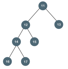
The above tree is a degenerate binary tree because all the nodes have only one child. It is also known as a right-skewed tree as all the nodes have a right child only.
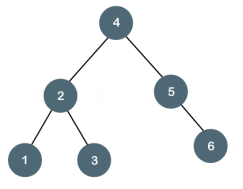
The above tree is also a degenerate binary tree because all the nodes have only one child. It is also known as a left-skewed tree as all the nodes have a left child only. Balanced Binary Tree The balanced binary tree is a tree in which both the left and right trees differ by atmost 1. For example, AVL and Red-Black trees are balanced binary tree. Let's understand the balanced binary tree through examples.
The above tree is a balanced binary tree because the difference between the left subtree and right subtree is zero.
The above tree is not a balanced binary tree because the difference between the left subtree and the right subtree is greater than 1. |
Binary Tree Implementation
A Binary tree is implemented with the help of pointers. The first node in the tree is represented by the root pointer. Each node in the tree consists of three parts, i.e., data, left pointer and right pointer. To create a binary tree, we first need to create the node. We will create the node of user-defined as shown below:
- struct node
- {
- int data,
- struct node *left, *right;
- }
In the above structure, data is the value, left pointer contains the address of the left node, and right pointer contains the address of the right node.
Binary Tree program in C
- #include<stdio.h>
- struct node
- {
- int data;
- struct node *left, *right;
- }
- void main()
- {
- struct node *root;
- root = create();
- }
- struct node *create()
- {
- struct node *temp;
- int data;
- temp = (struct node *)malloc(sizeof(struct node));
- printf("Press 0 to exit");
- printf("\nPress 1 for new node");
- printf("Enter your choice : ");
- scanf("%d", &choice);
- if(choice==0)
- {
- return 0;
- }
- else
- {
- printf("Enter the data:");
- scanf("%d", &data);
- temp->data = data;
- printf("Enter the left child of %d", data);
- temp->left = create();
- printf("Enter the right child of %d", data);
- temp->right = create();
- return temp;
- }
- }
The above code is calling the create() function recursively and creating new node on each recursive call. When all the nodes are created, then it forms a binary tree structure. The process of visiting the nodes is known as tree traversal. There are three types traversals used to visit a node:
- Inorder traversal
- Preorder traversal
- Postorder traversal
Traversal is a process to visit all the nodes of a tree and may print their values too. Because, all nodes are connected via edges (links) we always start from the root (head) node. That is, we cannot randomly access a node in a tree. There are three ways which we use to traverse a tree −
- In-order Traversal
- Pre-order Traversal
- Post-order Traversal
Generally, we traverse a tree to search or locate a given item or key in the tree or to print all the values it contains.
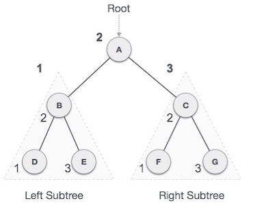
In this traversal method, the left subtree is visited first, then the root and later the right sub-tree. We should always remember that every node may represent a subtree itself.
If a binary tree is traversed in-order, the output will produce sorted key values in an ascending order.
|
Fig 7 - Inorder
We start from A, and following in-order traversal, we move to its left subtree B. B is also traversed in-order. The process goes on until all the nodes are visited. The output of inorder traversal of this tree will be −
D → B → E → A → F → C → G
Until all nodes are traversed −
Step 1 − Recursively traverse left subtree.
Step 2 − Visit root node.
Step 3 − Recursively traverse right subtree.
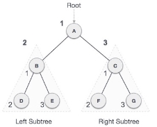
In this traversal method, the root node is visited first, then the left subtree and finally the right subtree.
|
Fig 8 – Pre order
We start from A, and following pre-order traversal, we first visit A itself and then move to its left subtree B. B is also traversed pre-order. The process goes on until all the nodes are visited. The output of pre-order traversal of this tree will be −
A → B → D → E → C → F → G
Until all nodes are traversed −
Step 1 − Visit root node.
Step 2 − Recursively traverse left subtree.
Step 3 − Recursively traverse right subtree.
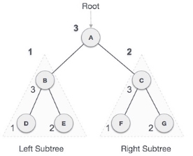
In this traversal method, the root node is visited last, hence the name. First we traverse the left subtree, then the right subtree and finally the root node.
|
Fig 9 – Post order
We start from A, and following Post-order traversal, we first visit the left subtree B. B is also traversed post-order. The process goes on until all the nodes are visited. The output of post-order traversal of this tree will be −
D → E → B → F → G → C → A
Until all nodes are traversed −
Step 1 − Recursively traverse left subtree.
Step 2 − Recursively traverse right subtree.
Step 3 − Visit root node.
Traversal is a process to visit all the nodes of a tree and may print their values too. Because, all nodes are connected via edges (links) we always start from the root (head) node. That is, we cannot random access a node in a tree. There are three ways which we use to traverse a tree −
- In-order Traversal
- Pre-order Traversal
- Post-order Traversal
We shall now look at the implementation of tree traversal in C programming language here using the following binary tree −
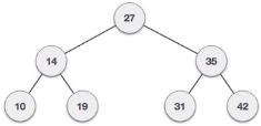
Fig 10 - Example
#include <stdio.h>
#include <stdlib.h>
struct node {
int data;
struct node *leftChild;
struct node *rightChild;
};
struct node *root = NULL;
void insert(int data) {
struct node *tempNode = (struct node*) malloc(sizeof(struct node));
struct node *current;
struct node *parent;
tempNode->data = data;
tempNode->leftChild = NULL;
tempNode->rightChild = NULL;
//if tree is empty
if(root == NULL) {
root = tempNode;
} else {
current = root;
parent = NULL;
while(1) {
parent = current;
//go to left of the tree
if(data < parent->data) {
current = current->leftChild;
//insert to the left
if(current == NULL) {
parent->leftChild = tempNode;
return;
}
} //go to right of the tree
else {
current = current->rightChild;
//insert to the right
if(current == NULL) {
parent->rightChild = tempNode;
return;
}
}
}
}
}
struct node* search(int data) {
struct node *current = root;
printf("Visiting elements: ");
while(current->data != data) {
if(current != NULL)
printf("%d ",current->data);
//go to left tree
if(current->data > data) {
current = current->leftChild;
}
//else go to right tree
else {
current = current->rightChild;
}
//not found
if(current == NULL) {
return NULL;
}
}
return current;
}
void pre_order_traversal(struct node* root) {
if(root != NULL) {
printf("%d ",root->data);
pre_order_traversal(root->leftChild);
pre_order_traversal(root->rightChild);
}
}
void inorder_traversal(struct node* root) {
if(root != NULL) {
inorder_traversal(root->leftChild);
printf("%d ",root->data);
inorder_traversal(root->rightChild);
}
}
void post_order_traversal(struct node* root) {
if(root != NULL) {
post_order_traversal(root->leftChild);
post_order_traversal(root->rightChild);
printf("%d ", root->data);
}
}
int main() {
int i;
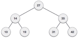
int array[7] = { 27, 14, 35, 10, 19, 31, 42 };
for(i = 0; i < 7; i++)
insert(array[i]);
i = 31;
struct node * temp = search(i);
if(temp != NULL) {
printf("[%d] Element found.", temp->data);
printf("\n");
}else {
printf("[ x ] Element not found (%d).\n", i);
}
i = 15;
temp = search(i);
if(temp != NULL) {
printf("[%d] Element found.", temp->data);
printf("\n");
}else {
printf("[ x ] Element not found (%d).\n", i);
}
printf("\nPreorder traversal: ");
pre_order_traversal(root);
printf("\nInorder traversal: ");
inorder_traversal(root);
printf("\nPost order traversal: ");
post_order_traversal(root);
return 0;
}
If we compile and run the above program, it will produce the following result −
Visiting elements: 27 35 [31] Element found.
Visiting elements: 27 14 19 [ x ] Element not found (15).
Preorder traversal: 27 14 10 19 35 31 42
Inorder traversal: 10 14 19 27 31 35 42
Post order traversal: 10 19 14 31 42 35 27
Tree represents the nodes connected by edges. We will discuss binary tree or binary search tree specifically.
Binary Tree is a special datastructure used for data storage purposes. A binary tree has a special condition that each node can have a maximum of two children. A binary tree has the benefits of both an ordered array and a linked list as search is as quick as in a sorted array and insertion or deletion operation are as fast as in linked list.
|
Fig 11 - Binary Tree
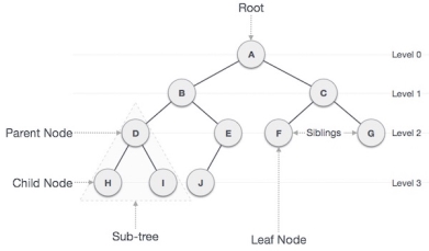
Following are the important terms with respect to tree.
- Path − Path refers to the sequence of nodes along the edges of a tree.
- Root − The node at the top of the tree is called root. There is only one root per tree and one path from the root node to any node.
- Parent − Any node except the root node has one edge upward to a node called parent.
- Child − The node below a given node connected by its edge downward is called its child node.
- Leaf − The node which does not have any child node is called the leaf node.
- Subtree − Subtree represents the descendants of a node.
- Visiting − Visiting refers to checking the value of a node when control is on the node.
- Traversing − Traversing means passing through nodes in a specific order.
- Levels − Level of a node represents the generation of a node. If the root node is at level 0, then its next child node is at level 1, its grandchild is at level 2, and so on.
- keys − Key represents a value of a node based on which a search operation is to be carried out for a node.
Binary Search Tree Representation
Binary Search tree exhibits a special behavior. A node's left child must have a value less than its parent's value and the node's right child must have a value greater than its parent value.
|
Fig 12 - Binary Search tree
We're going to implement tree using node object and connecting them through references.
The code to write a tree node would be similar to what is given below. It has a data part and references to its left and right child nodes.
struct node {
int data;
struct node *leftChild;
struct node *rightChild;
};
In a tree, all nodes share common construct.
The basic operations that can be performed on a binary search tree data structure, are the following −
- Insert − Inserts an element in a tree/create a tree.
- Search − Searches an element in a tree.
- Preorder Traversal − Traverses a tree in a pre-order manner.
- Inorder Traversal − Traverses a tree in an in-order manner.
- Postorder Traversal − Traverses a tree in a post-order manner.
We shall learn creating (inserting into) a tree structure and searching a data item in a tree in this chapter. We shall learn about tree traversing methods in the coming chapter.
The very first insertion creates the tree. Afterwards, whenever an element is to be inserted, first locate its proper location. Start searching from the root node, then if the data is less than the key value, search for the empty location in the left subtree and insert the data. Otherwise, search for the empty location in the right subtree and insert the data.
If root is NULL
then create root node
return
If root exists then
compare the data with node.data
while until insertion position is located
If data is greater than node.data
goto right subtree
else
goto left subtree
endwhile
insert data
end If
The implementation of insert function should look like this −
void insert(int data) {
struct node *tempNode = (struct node*) malloc(sizeof(struct node));
struct node *current;
struct node *parent;
tempNode->data = data;
tempNode->leftChild = NULL;
tempNode->rightChild = NULL;
//if tree is empty, create root node
if(root == NULL) {
root = tempNode;
} else {
current = root;
parent = NULL;
while(1) {
parent = current;
//go to left of the tree
if(data < parent->data) {
current = current->leftChild;
//insert to the left
if(current == NULL) {
parent->leftChild = tempNode;
return;
}
}
//go to right of the tree
else {
current = current->rightChild;
//insert to the right
if(current == NULL) {
parent->rightChild = tempNode;
return;
}
}
}
}
}
Whenever an element is to be searched, start searching from the root node, then if the data is less than the key value, search for the element in the left subtree. Otherwise, search for the element in the right subtree. Follow the same algorithm for each node.
If root.data is equal to search.data
return root
else
while data not found
If data is greater than node.data
goto right subtree
else
goto left subtree
If data found
return node
endwhile
return data not found
end if
The implementation of this algorithm should look like this.
struct node* search(int data) {
struct node *current = root;
printf("Visiting elements: ");
while(current->data != data) {
if(current != NULL)
printf("%d ",current->data);
//go to left tree
if(current->data > data) {
current = current->leftChild;
}
//else go to right tree
else {
current = current->rightChild;
}
//not found
if(current == NULL) {
return NULL;
}
return current;
}
}
Key takeaway
The Binary tree means that the node can have maximum two children. Here, binary name itself suggests that 'two'; therefore, each node can have either 0, 1 or 2 children.
AVL Tree is invented by GM Adelson - Velsky and EM Landis in 1962. The tree is named AVL in honour of its inventors.
AVL Tree can be defined as height balanced binary search tree in which each node is associated with a balance factor which is calculated by subtracting the height of its right sub-tree from that of its left sub-tree.
Tree is said to be balanced if balance factor of each node is in between -1 to 1, otherwise, the tree will be unbalanced and need to be balanced.
Balance Factor (k) = height (left(k)) - height (right(k))
If balance factor of any node is 1, it means that the left sub-tree is one level higher than the right sub-tree.
If balance factor of any node is 0, it means that the left sub-tree and right sub-tree contain equal height.
If balance factor of any node is -1, it means that the left sub-tree is one level lower than the right sub-tree.
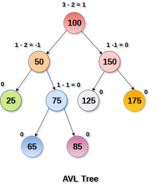
An AVL tree is given in the following figure. We can see that, balance factor associated with each node is in between -1 and +1. therefore, it is an example of AVL tree.
|
Fig 13 – AVL Tree
Algorithm | Average case | Worst case |
Space | o(n) | o(n) |
Search | o(log n) | o(log n) |
Insert | o(log n) | o(log n) |
Delete | o(log n) | o(log n) |
Due to the fact that, AVL tree is also a binary search tree therefore, all the operations are performed in the same way as they are performed in a binary search tree. Searching and traversing do not lead to the violation in property of AVL tree. However, insertion and deletion are the operations which can violate this property and therefore, they need to be revisited.
SN | Operation | Description |
1 | Insertion | Insertion in AVL tree is performed in the same way as it is performed in a binary search tree. However, it may lead to violation in the AVL tree property and therefore the tree may need balancing. The tree can be balanced by applying rotations. |
2 | Deletion | Deletion can also be performed in the same way as it is performed in a binary search tree. Deletion may also disturb the balance of the tree therefore, various types of rotations are used to rebalance the tree. |
AVL tree controls the height of the binary search tree by not letting it to be skewed. The time taken for all operations in a binary search tree of height h is O(h). However, it can be extended to O(n) if the BST becomes skewed (i.e. worst case). By limiting this height to log n, AVL tree imposes an upper bound on each operation to be O(log n) where n is the number of nodes.
We perform rotation in AVL tree only in case if Balance Factor is other than -1, 0, and 1. There are basically four types of rotations which are as follows:
- L L rotation: Inserted node is in the left subtree of left subtree of A
- R R rotation : Inserted node is in the right subtree of right subtree of A
- L R rotation : Inserted node is in the right subtree of left subtree of A
- R L rotation : Inserted node is in the left subtree of right subtree of A
Where node A is the node whose balance Factor is other than -1, 0, 1.
The first two rotations LL and RR are single rotations and the next two rotations LR and RL are double rotations. For a tree to be unbalanced, minimum height must be at least 2, Let us understand each rotation
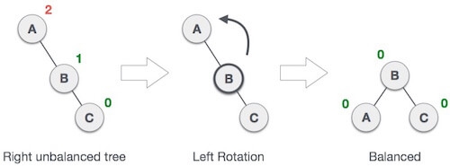
When BST becomes unbalanced, due to a node is inserted into the right subtree of the right subtree of A, then we perform RR rotation, RR rotation is an anticlockwise rotation, which is applied on the edge below a node having balance factor -2
|
In above example, node A has balance factor -2 because a node C is inserted in the right subtree of A right subtree. We perform the RR rotation on the edge below A.
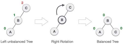
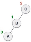
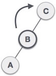
When BST becomes unbalanced, due to a node is inserted into the left subtree of the left subtree of C, then we perform LL rotation, LL rotation is clockwise rotation, which is applied on the edge below a node having balance factor 2.
|
In above example, node C has balance factor 2 because a node A is inserted in the left subtree of C left subtree. We perform the LL rotation on the edge below A.
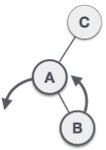
Double rotations are bit tougher than single rotation which has already explained above. LR rotation = RR rotation + LL rotation, i.e., first RR rotation is performed on subtree and then LL rotation is performed on full tree, by full tree we mean the first node from the path of inserted node whose balance factor is other than -1, 0, or 1.
Let us understand each and every step very clearly:
State | Action |
| A node B has been inserted into the right subtree of A the left subtree of C, because of which C has become an unbalanced node having balance factor 2. This case is L R rotation where: Inserted node is in the right subtree of left subtree of C |
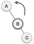
| As LR rotation = RR + LL rotation, hence RR (anticlockwise) on subtree rooted at A is performed first. By doing RR rotation, node A, has become the left subtree of B. |
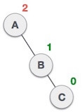
| After performing RR rotation, node C is still unbalanced, i.e., having balance factor 2, as inserted node A is in the left of left of C |
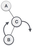
| Now we perform LL clockwise rotation on full tree, i.e. on node C. node C has now become the right subtree of node B, A is left subtree of B |
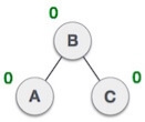
| Balance factor of each node is now either -1, 0, or 1, i.e. BST is balanced now. |
As already discussed, that double rotations are bit tougher than single rotation which has already explained above. R L rotation = LL rotation + RR rotation, i.e., first LL rotation is performed on subtree and then RR rotation is performed on full tree, by full tree we mean the first node from the path of inserted node whose balance factor is other than -1, 0, or 1.
State | Action |
| A node B has been inserted into the left subtree of C the right subtree of A, because of which A has become an unbalanced node having balance factor - 2. This case is RL rotation where: Inserted node is in the left subtree of right subtree of A |
| As RL rotation = LL rotation + RR rotation, hence, LL (clockwise) on subtree rooted at C is performed first. By doing RR rotation, node C has become the right subtree of B. |
| After performing LL rotation, node A is still unbalanced, i.e. having balance factor -2, which is because of the right-subtree of the right-subtree node A. |
| Now we perform RR rotation (anticlockwise rotation) on full tree, i.e. on node A. node C has now become the right subtree of node B, and node A has become the left subtree of B. |
| Balance factor of each node is now either -1, 0, or 1, i.e., BST is balanced now. |
Q: Construct an AVL tree having the following elements
H, I, J, B, A, E, C, F, D, G, K, L
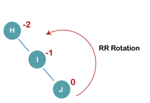
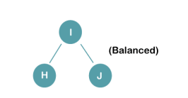
1. Insert H, I, J
|
On inserting the above elements, especially in the case of H, the BST becomes unbalanced as the Balance Factor of H is -2. Since the BST is right-skewed, we will perform RR Rotation on node H.
The resultant balance tree is:
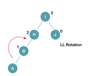
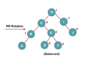
2. Insert B, A
|
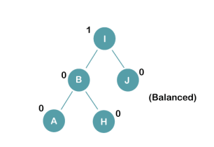
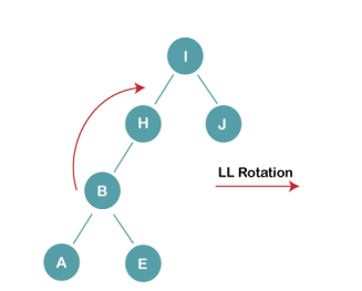
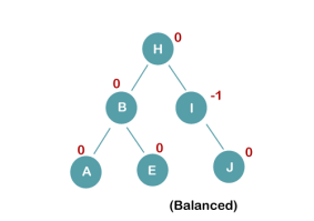
On inserting the above elements, especially in case of A, the BST becomes unbalanced as the Balance Factor of H and I is 2, we consider the first node from the last inserted node i.e. H. Since the BST from H is left-skewed, we will perform LL Rotation on node H.
The resultant balance tree is:
|
3. Insert E
|
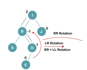
On inserting E, BST becomes unbalanced as the Balance Factor of I is 2, since if we travel from E to I we find that it is inserted in the left subtree of right subtree of I, we will perform LR Rotation on node I. LR = RR + LL rotation
3 a) We first perform RR rotation on node B
The resultant tree after RR rotation is:
|
3b) We first perform LL rotation on the node I
The resultant balanced tree after LL rotation is:
|
4. Insert C, F, D
|
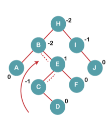
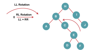
On inserting C, F, D, BST becomes unbalanced as the Balance Factor of B and H is -2, since if we travel from D to B we find that it is inserted in the right subtree of left subtree of B, we will perform RL Rotation on node I. RL = LL + RR rotation.
4a) We first perform LL rotation on node E
The resultant tree after LL rotation is:
|
4b) We then perform RR rotation on node B
The resultant balanced tree after RR rotation is:
|
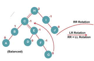
5. Insert G
|
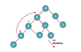
On inserting G, BST become unbalanced as the Balance Factor of H is 2, since if we travel from G to H, we find that it is inserted in the left subtree of right subtree of H, we will perform LR Rotation on node I. LR = RR + LL rotation.
5 a) We first perform RR rotation on node C
The resultant tree after RR rotation is:
|
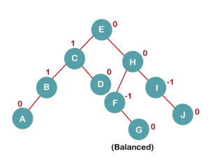
5 b) We then perform LL rotation on node H
The resultant balanced tree after LL rotation is:
|
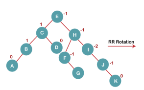
6. Insert K
|
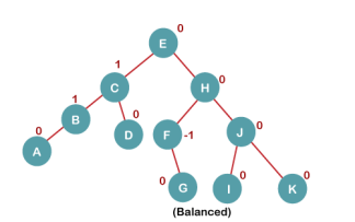
On inserting K, BST becomes unbalanced as the Balance Factor of I is -2. Since the BST is right-skewed from I to K, hence we will perform RR Rotation on the node I.
The resultant balanced tree after RR rotation is:
|
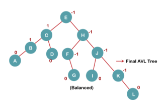
7. Insert L
On inserting the L tree is still balanced as the Balance Factor of each node is now either, -1, 0, +1. Hence the tree is a Balanced AVL tree
|
Key takeaway
AVL Tree is invented by GM Adelson - Velsky and EM Landis in 1962. The tree is named AVL in honour of its inventors.
AVL Tree can be defined as height balanced binary search tree in which each node is associated with a balance factor which is calculated by subtracting the height of its right sub-tree from that of its left sub-tree.
Tree is said to be balanced if balance factor of each node is in between -1 to 1, otherwise, the tree will be unbalanced and need to be balanced.
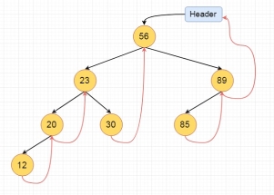
Here we will see the threaded binary tree data structure. We know that the binary tree nodes may have at most two children. But if they have only one children, or no children, the link part in the linked list representation remains null. Using threaded binary tree representation, we can reuse that empty links by making some threads.
If one node has some vacant left or right child area, that will be used as thread. There are two types of threaded binary tree. The single threaded tree or fully threaded binary tree. In single threaded mode, there are another two variations. Left threaded and right threaded.
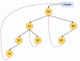
In the left threaded mode if some node has no left child, then the left pointer will point to its inorder predecessor, similarly in the right threaded mode if some node has no right child, then the right pointer will point to its inorder successor. In both cases, if no successor or predecessor is present, then it will point to header node.
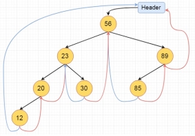
For fully threaded binary tree, each node has five fields. Three fields like normal binary tree node, another two fields to store Boolean value to denote whether link of that side is actual link or thread.
Fig 14 - Example These are the examples of left and right threaded tree
Fig 15 - Example
|
This is the fully threaded binary tree
|
Fig 16 - Fully threaded binary tree
Key takeaway
Here we will see the threaded binary tree data structure. We know that the binary tree nodes may have at most two children. But if they have only one children, or no children, the link part in the linked list representation remains null. Using threaded binary tree representation, we can reuse that empty links by making some threads.
If one node has some vacant left or right child area, that will be used as thread. There are two types of threaded binary tree. The single threaded tree or fully threaded binary tree. In single threaded mode, there are another two variations. Left threaded and right threaded.
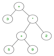
The expression tree is a binary tree in which each internal node corresponds to the operator and each leaf node corresponds to the operand so for example expression tree for 3 + ((5+9)*2) would be:
|
Fig 17 – Expression tree
Inorder traversal of expression tree produces infix version of given postfix expression (same with postorder traversal it gives postfix expression)
Evaluating the expression represented by an expression tree:
Let t be the expression tree
If t is not null then
If t.value is operand then
Return t.value
A = solve(t.left)
B = solve(t.right)
// calculate applies operator 't.value'
// on A and B, and returns value
Return calculate(A, B, t.value)
Construction of Expression Tree:
Now For constructing an expression tree we use a stack. We loop through input expression and do the following for every character.
- If a character is an operand push that into the stack
- If a character is an operator pop two values from the stack make them its child and push the current node again.
In the end, the only element of the stack will be the root of an expression tree.
Below is the implementation of the above approach:
// C++ program for expression tree #include<bits/stdc++.h> using namespace std;
// An expression tree node struct et { char value; et* left, *right; };
// A utility function to check if 'c' // is an operator bool isOperator(char c) { if (c == '+' || c == '-' || c == '*' || c == '/' || c == '^') return true; return false; }
// Utility function to do inorder traversal void inorder(et *t) { if(t) { inorder(t->left); printf("%c ", t->value); inorder(t->right); } }
// A utility function to create a new node et* newNode(char v) { et *temp = new et; temp->left = temp->right = NULL; temp->value = v; return temp; };
// Returns root of constructed tree for given // postfix expression et* constructTree(char postfix[]) { stack<et *> st; et *t, *t1, *t2;
// Traverse through every character of // input expression for (int i=0; i<strlen(postfix); i++) { // If operand, simply push into stack if (!isOperator(postfix[i])) { t = newNode(postfix[i]); st.push(t); } else // operator { t = newNode(postfix[i]);
// Pop two top nodes t1 = st.top(); // Store top st.pop(); // Remove top t2 = st.top(); st.pop();
// make them children t->right = t1; t->left = t2;
// Add this subexpression to stack st.push(t); } }
// only element will be root of expression // tree t = st.top(); st.pop();
return t; }
// Driver program to test above int main() { char postfix[] = "ab+ef*g*-"; et* r = constructTree(postfix); printf("infix expression is \n"); inorder(r); return 0; } |
Output
infix expression is
a + b - e * f * g
Key takeaway
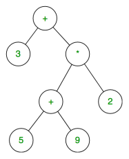
The expression tree is a binary tree in which each internal node corresponds to the operator and each leaf node corresponds to the operand so for example expression tree for 3 + ((5+9)*2) would be:
|
Inorder traversal of expression tree produces infix version of given postfix expression (same with postorder traversal it gives postfix expression)
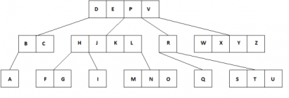
A multiway tree is defined as a tree that can have more than two children. If a multiway tree can have maximum m children, then this tree is called as multiway tree of order m (or an m-way tree).
As with the other trees that have been studied, the nodes in an m-way tree will be made up of m-1 key fields and pointers to children.
multiway tree of order 5
|
Fig 18 – Multiway Tree
To make the processing of m-way trees easier some type of constraint or order will be imposed on the keys within each node, resulting in a multiway search tree of order m (or an m-way search tree). By definition an m-way search tree is a m-way tree in which following condition should be satisfied −
- Each node is associated with m children and m-1 key fields
- The keys in each node are arranged in ascending order.
- The keys in the first j children are less than the j-th key.
- The keys in the last m-j children are higher than the j-th key.
Key takeaway
A multiway tree is defined as a tree that can have more than two children. If a multiway tree can have maximum m children, then this tree is called as multiway tree of order m (or an m-way tree).
As with the other trees that have been studied, the nodes in an m-way tree will be made up of m-1 key fields and pointers to children.
B+ Tree is an extension of B Tree which allows efficient insertion, deletion and search operations.
In B Tree, Keys and records both can be stored in the internal as well as leaf nodes. Whereas, in B+ tree, records (data) can only be stored on the leaf nodes while internal nodes can only store the key values.
The leaf nodes of a B+ tree are linked together in the form of a singly linked lists to make the search queries more efficient.
B+ Tree are used to store the large amount of data which can not be stored in the main memory. Due to the fact that, size of main memory is always limited, the internal nodes (keys to access records) of the B+ tree are stored in the main memory whereas, leaf nodes are stored in the secondary memory.
The internal nodes of B+ tree are often called index nodes. A B+ tree of order 3 is shown in the following figure.
|
Fig 19 – B+ Tree
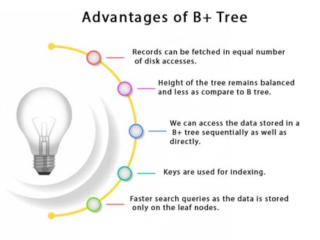
- Records can be fetched in equal number of disk accesses.
- Height of the tree remains balanced and less as compare to B tree.
- We can access the data stored in a B+ tree sequentially as well as directly.
- Keys are used for indexing.
- Faster search queries as the data is stored only on the leaf nodes.
|
Fig 20 – Advantages of B+ Tree
SN | B Tree | B+ Tree |
1 | Search keys can not be repeatedly stored. | Redundant search keys can be present. |
2 | Data can be stored in leaf nodes as well as internal nodes | Data can only be stored on the leaf nodes. |
3 | Searching for some data is a slower process since data can be found on internal nodes as well as on the leaf nodes. | Searching is comparatively faster as data can only be found on the leaf nodes. |
4 | Deletion of internal nodes are so complicated and time consuming. | Deletion will never be a complexed process since element will always be deleted from the leaf nodes. |
5 | Leaf nodes can not be linked together. | Leaf nodes are linked together to make the search operations more efficient. |
Step 1: Insert the new node as a leaf node Step 2: If the leaf doesn't have required space, split the node and copy the middle node to the next index node. Step 3: If the index node doesn't have required space, split the node and copy the middle element to the next index page. Insert the value 195 into the B+ tree of order 5 shown in the following figure.
195 will be inserted in the right sub-tree of 120 after 190. Insert it at the desired position.
The node contains greater than the maximum number of elements i.e. 4, therefore split it and place the median node up to the parent.
Now, the index node contains 6 children and 5 keys which violates the B+ tree properties, therefore we need to split it, shown as follows.
Step 1: Delete the key and data from the leaves. Step 2: if the leaf node contains less than minimum number of elements, merge down the node with its sibling and delete the key in between them. Step 3: if the index node contains less than minimum number of elements, merge the node with the sibling and move down the key in between them. Delete the key 200 from the B+ Tree shown in the following figure.
200 is present in the right sub-tree of 190, after 195. delete it.
Merge the two nodes by using 195, 190, 154 and 129.
Now, element 120 is the single element present in the node which is violating the B+ Tree properties. Therefore, we need to merge it by using 60, 78, 108 and 120. Now, the height of B+ tree will be decreased by 1.
|
Key takeaway
B+ Tree is an extension of B Tree which allows efficient insertion, deletion and search operations.
In B Tree, Keys and records both can be stored in the internal as well as leaf nodes. Whereas, in B+ tree, records (data) can only be stored on the leaf nodes while internal nodes can only store the key values.
The leaf nodes of a B+ tree are linked together in the form of a singly linked lists to make the search queries more efficient.
Heap is a special case of balanced binary tree data structure where the root-node key is compared with its children and arranged accordingly. If α has child node β then −
key(α) ≥ key(β)
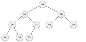
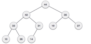
For Input → 35 33 42 10 14 19 27 44 26 31 Min-Heap − Where the value of the root node is less than or equal to either of its children.
Fig 21 – Min Heap Max-Heap − Where the value of the root node is greater than or equal to either of its children.
Fig 22 – Max Heap Both trees are constructed using the same input and order of arrival. |
Max Heap Construction Algorithm
We shall use the same example to demonstrate how a Max Heap is created. The procedure to create Min Heap is similar but we go for min values instead of max values.
We are going to derive an algorithm for max heap by inserting one element at a time. At any point of time, heap must maintain its property. While insertion, we also assume that we are inserting a node in an already heapified tree.
Step 1 − Create a new node at the end of heap.
Step 2 − Assign new value to the node.
Step 3 − Compare the value of this child node with its parent.
Step 4 − If value of parent is less than child, then swap them.
Step 5 − Repeat step 3 & 4 until Heap property holds.
Note − In Min Heap construction algorithm, we expect the value of the parent node to be less than that of the child node.
Let's understand Max Heap construction by an animated illustration. We consider the same input sample that we used earlier.
Let us derive an algorithm to delete from max heap. Deletion in Max (or Min) Heap always happens at the root to remove the Maximum (or minimum) value.
Step 1 − Remove root node.
Step 2 − Move the last element of last level to root.
Step 3 − Compare the value of this child node with its parent.
Step 4 − If value of parent is less than child, then swap them.
Step 5 − Repeat step 3 & 4 until Heap property holds.
|
Fig 23 – Deletion Algorithm
Key takeaway
Heap is a special case of balanced binary tree data structure where the root-node key is compared with its children and arranged accordingly. If α has child node β then −
key(α) ≥ key(β)
As the value of parent is greater than that of child, this property generates Max Heap. Based on this criteria, a heap can be of two types −
For Input → 35 33 42 10 14 19 27 44 26 31
Reference
1 Data structure & algorithm analysis in C by Mark Allen Weiss published by Pearson Education (LPE)
2 Introduction to Data structure in C by A.N. Kathie published by Pearson Education (LPE)
