UNIT-6
Graphs & Hashing
A graph can be defined as group of vertices and edges that are used to connect these vertices. A graph can be seen as a cyclic tree, where the vertices (Nodes) maintain any complex relationship among them instead of having parent child relationship.
A graph G can be defined as an ordered set G(V, E) where V(G) represents the set of vertices and E(G) represents the set of edges which are used to connect these vertices.
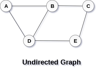
A Graph G(V, E) with 5 vertices (A, B, C, D, E) and six edges ((A,B), (B,C), (C,E), (E,D), (D,B), (D,A)) is shown in the following figure.
|
Fig 1 – Undirected graph
A graph can be directed or undirected. However, in an undirected graph, edges are not associated with the directions with them. An undirected graph is shown in the above figure since its edges are not attached with any of the directions. If an edge exists between vertex A and B then the vertices can be traversed from B to A as well as A to B.
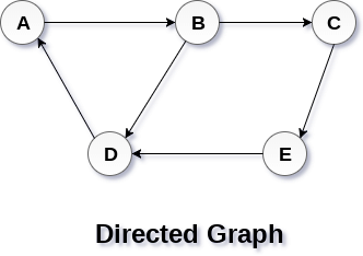
In a directed graph, edges form an ordered pair. Edges represent a specific path from some vertex A to another vertex B. Node A is called initial node while node B is called terminal node.
A directed graph is shown in the following figure.
|
Fig 2 – Directed graph
A path can be defined as the sequence of nodes that are followed in order to reach some terminal node V from the initial node U.
A path will be called as closed path if the initial node is same as terminal node. A path will be closed path if V0=VN.
If all the nodes of the graph are distinct with an exception V0=VN, then such path P is called as closed simple path.
A cycle can be defined as the path which has no repeated edges or vertices except the first and last vertices.
A connected graph is the one in which some path exists between every two vertices (u, v) in V. There are no isolated nodes in connected graph.
A complete graph is the one in which every node is connected with all other nodes. A complete graph contain n(n-1)/2 edges where n is the number of nodes in the graph.
In a weighted graph, each edge is assigned with some data such as length or weight. The weight of an edge e can be given as w(e) which must be a positive (+) value indicating the cost of traversing the edge.
A digraph is a directed graph in which each edge of the graph is associated with some direction and the traversing can be done only in the specified direction.
An edge that is associated with the similar end points can be called as Loop.
If two nodes u and v are connected via an edge e, then the nodes u and v are called as neighbours or adjacent nodes.
A degree of a node is the number of edges that are connected with that node. A node with degree 0 is called as isolated node.
Key takeaway
A graph can be defined as group of vertices and edges that are used to connect these vertices. A graph can be seen as a cyclic tree, where the vertices (Nodes) maintain any complex relationship among them instead of having parent child relationship.
By Graph representation, we simply mean the technique which is to be used in order to store some graph into the computer's memory.
There are two ways to store Graph into the computer's memory. In this part of this tutorial, we discuss each one of them in detail.
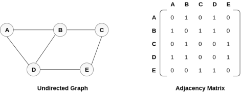
In sequential representation, we use adjacency matrix to store the mapping represented by vertices and edges. In adjacency matrix, the rows and columns are represented by the graph vertices. A graph having n vertices, will have a dimension n x n.
An entry Mij in the adjacency matrix representation of an undirected graph G will be 1 if there exists an edge between Vi and Vj.
An undirected graph and its adjacency matrix representation is shown in the following figure.
|
Fig 3 – Undirected graph and its adjacency matrix
In the above figure, we can see the mapping among the vertices (A, B, C, D, E) is represented by using the adjacency matrix which is also shown in the figure.
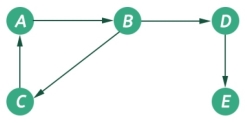
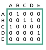
There exists different adjacency matrices for the directed and undirected graph. In directed graph, an entry Aij will be 1 only when there is an edge directed from Vi to Vj.
A directed graph and its adjacency matrix representation is shown in the following figure.
|
Fig 4 - Directed graph and its adjacency matrix
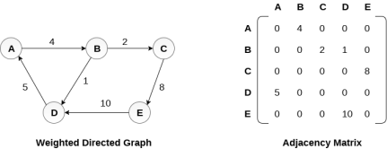
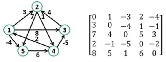
Representation of weighted directed graph is different. Instead of filling the entry by 1, the Non- zero entries of the adjacency matrix are represented by the weight of respective edges.
The weighted directed graph along with the adjacency matrix representation is shown in the following figure.
|
Fig 5 - Weighted directed graph
In the linked representation, an adjacency list is used to store the Graph into the computer's memory.
Consider the undirected graph shown in the following figure and check the adjacency list representation.
|
Fig 6 - Undirected graph in adjacency list
An adjacency list is maintained for each node present in the graph which stores the node value and a pointer to the next adjacent node to the respective node. If all the adjacent nodes are traversed then store the NULL in the pointer field of last node of the list. The sum of the lengths of adjacency lists is equal to the twice of the number of edges present in an undirected graph.
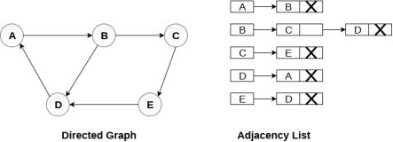
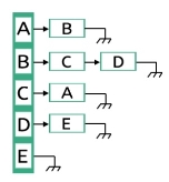
Consider the directed graph shown in the following figure and check the adjacency list representation of the graph.
|
Fig 7 - Directed graph in adjacency list
In a directed graph, the sum of lengths of all the adjacency lists is equal to the number of edges present in the graph.
In the case of weighted directed graph, each node contains an extra field that is called the weight of the node. The adjacency list representation of a directed graph is shown in the following figure.
|
Fig 8 - weighted directed graph
Key takeaway
By Graph representation, we simply mean the technique which is to be used in order to store some graph into the computer's memory.
There are two ways to store Graph into the computer's memory.
Floyd-Warshall algorithm is used to find all pair shortest path problem from a given weighted graph. As a result of this algorithm, it will generate a matrix, which will represent the minimum distance from any node to all other nodes in the graph.
|
Fig 9 - Example
At first, the output matrix is the same as the given cost matrix of the graph. After that, the output matrix will be updated with all vertices k as the intermediate vertex.
The time complexity of this algorithm is O(V^3), where V is the number of vertices in the graph.
Input: The cost matrix of the graph.
0 3 6 ∞ ∞ ∞ ∞
3 0 2 1 ∞ ∞ ∞
6 2 0 1 4 2 ∞
∞ 1 1 0 2 ∞ 4
∞ ∞ 4 2 0 2 1
∞ ∞ 2 ∞ 2 0 1
∞ ∞ ∞ 4 1 1 0
Output:
Matrix of all pair shortest path.
0 3 4 5 6 7 7
3 0 2 1 3 4 4
4 2 0 1 3 2 3
5 1 1 0 2 3 3
6 3 3 2 0 2 1
7 4 2 3 2 0 1
7 4 3 3 1 1 0
floydWarshal(cost)
Input − The cost matrix of given Graph.
Output: Matrix to for shortest path between any vertex to any vertex.
Begin
for k := 0 to n, do
for i := 0 to n, do
for j := 0 to n, do
if cost[i,k] + cost[k,j] < cost[i,j], then
cost[i,j] := cost[i,k] + cost[k,j]
done
done
done
display the current cost matrix
End
#include<iostream>
#include<iomanip>
#define NODE 7
#define INF 999
using namespace std;
//Cost matrix of the graph
int costMat[NODE][NODE] = {
{0, 3, 6, INF, INF, INF, INF},
{3, 0, 2, 1, INF, INF, INF},
{6, 2, 0, 1, 4, 2, INF},
{INF, 1, 1, 0, 2, INF, 4},
{INF, INF, 4, 2, 0, 2, 1},
{INF, INF, 2, INF, 2, 0, 1},
{INF, INF, INF, 4, 1, 1, 0}
};
void floydWarshal() {
int cost[NODE][NODE]; //defind to store shortest distance from any node to any node
for(int i = 0; i<NODE; i++)
for(int j = 0; j<NODE; j++)
cost[i][j] = costMat[i][j]; //copy costMatrix to new matrix
for(int k = 0; k<NODE; k++) {
for(int i = 0; i<NODE; i++)
for(int j = 0; j<NODE; j++)
if(cost[i][k]+cost[k][j] < cost[i][j])
cost[i][j] = cost[i][k]+cost[k][j];
}
cout << "The matrix:" << endl;
for(int i = 0; i<NODE; i++) {
for(int j = 0; j<NODE; j++)
cout << setw(3) << cost[i][j];
cout << endl;
}
}
int main() {
floydWarshal();
}
The matrix:
0 3 5 4 6 7 7
3 0 2 1 3 4 4
5 2 0 1 3 2 3
4 1 1 0 2 3 3
6 3 3 2 0 2 1
7 4 2 3 2 0 1
7 4 3 3 1 1 0
Key takeaway
Floyd-Warshall algorithm is used to find all pair shortest path problem from a given weighted graph. As a result of this algorithm, it will generate a matrix, which will represent the minimum distance from any node to all other nodes in the graph.
Dijkstra’s algorithm solves the single-source shortest-paths problem on a directed weighted graph G = (V, E), where all the edges are non-negative (i.e., w(u, v) ≥ 0 for each edge (u, v) Є E).
In the following algorithm, we will use one function Extract-Min(), which extracts the node with the smallest key.
Algorithm: Dijkstra’s-Algorithm (G, w, s)
for each vertex v Є G.V
v.d := ∞
v.∏ := NIL
s.d := 0
S := Ф
Q := G.V
while Q ≠ Ф
u := Extract-Min (Q)
S := S U {u}
for each vertex v Є G.adj[u]
if v.d > u.d + w(u, v)
v.d := u.d + w(u, v)
v.∏ := u
The complexity of this algorithm is fully dependent on the implementation of Extract-Min function. If extract min function is implemented using linear search, the complexity of this algorithm is O(V2 + E).
In this algorithm, if we use min-heap on which Extract-Min() function works to return the node from Q with the smallest key, the complexity of this algorithm can be reduced further.
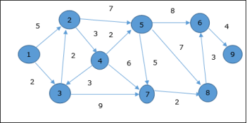
Let us consider vertex 1 and 9 as the start and destination vertex respectively. Initially, all the vertices except the start vertex are marked by ∞ and the start vertex is marked by 0.
Vertex | Initial | Step1 V1 | Step2 V3 | Step3 V2 | Step4 V4 | Step5 V5 | Step6 V7 | Step7 V8 | Step8 V6 |
1 | 0 | 0 | 0 | 0 | 0 | 0 | 0 | 0 | 0 |
2 | ∞ | 5 | 4 | 4 | 4 | 4 | 4 | 4 | 4 |
3 | ∞ | 2 | 2 | 2 | 2 | 2 | 2 | 2 | 2 |
4 | ∞ | ∞ | ∞ | 7 | 7 | 7 | 7 | 7 | 7 |
5 | ∞ | ∞ | ∞ | 11 | 9 | 9 | 9 | 9 | 9 |
6 | ∞ | ∞ | ∞ | ∞ | ∞ | 17 | 17 | 16 | 16 |
7 | ∞ | ∞ | 11 | 11 | 11 | 11 | 11 | 11 | 11 |
8 | ∞ | ∞ | ∞ | ∞ | ∞ | 16 | 13 | 13 | 13 |
9 | ∞ | ∞ | ∞ | ∞ | ∞ | ∞ | ∞ | ∞ | 20 |
Hence, the minimum distance of vertex 9 from vertex 1 is 20. And the path is
1→ 3→ 7→ 8→ 6→ 9
This path is determined based on predecessor information.
|
Fig 10 - Example
This algorithm solves the single source shortest path problem of a directed graph G = (V, E) in which the edge weights may be negative. Moreover, this algorithm can be applied to find the shortest path, if there does not exist any negative weighted cycle.
Algorithm: Bellman-Ford-Algorithm (G, w, s)
for each vertex v Є G.V
v.d := ∞
v.∏ := NIL
s.d := 0
for i = 1 to |G.V| - 1
for each edge (u, v) Є G.E
if v.d > u.d + w(u, v)
v.d := u.d +w(u, v)
v.∏ := u
for each edge (u, v) Є G.E
if v.d > u.d + w(u, v)
return FALSE
return TRUE
The first for loop is used for initialization, which runs in O(V) times. The next for loop runs |V - 1| passes over the edges, which takes O(E) times.
Hence, Bellman-Ford algorithm runs in O(V, E) time.
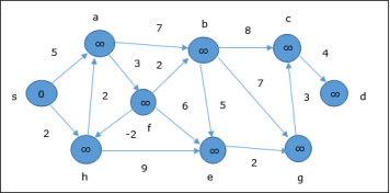
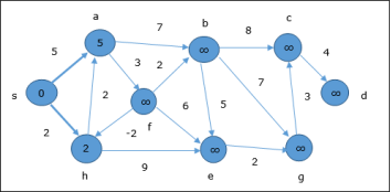
The following example shows how Bellman-Ford algorithm works step by step. This graph has a negative edge but does not have any negative cycle, hence the problem can be solved using this technique. At the time of initialization, all the vertices except the source are marked by ∞ and the source is marked by 0.
In the first step, all the vertices which are reachable from the source are updated by minimum cost. Hence, vertices a and h are updated.
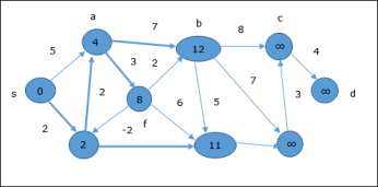
In the next step, vertices a, b, f and e are updated.
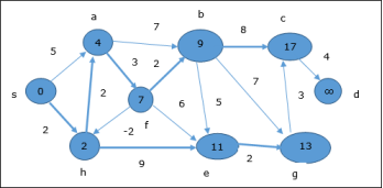
Following the same logic, in this step vertices b, f, c and g are updated.
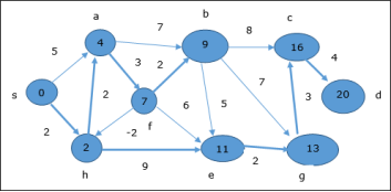
Here, vertices c and d are updated.
Hence, the minimum distance between vertex s and vertex d is 20. Based on the predecessor information, the path is s→ h→ e→ g→ c→ d |
Key takeaway
Dijkstra’s algorithm solves the single-source shortest-paths problem on a directed weighted graph G = (V, E), where all the edges are non-negative (i.e., w(u, v) ≥ 0 for each edge (u, v) Є E).
In the following algorithm, we will use one function Extract-Min(), which extracts the node with the smallest key.
The graph is a non-linear data structures. This represents data using nodes, and their relations using edges. A graph G has two sections. The vertices, and edges. Vertices are represented using set V, and Edges are represented as set E. So the graph notation is G(V,E). Let us see one example to get the idea.
|
Fig 11 - Example
In this graph, there are five vertices and five edges. The edges are directed. As an example, if we choose the edge connecting vertices B and D, the source vertex is B and destination is D. So we can move B to D but not move from D to B.
The graphs are non-linear, and it has no regular structure. To represent a graph in memory, there are few different styles. These styles are −
- Adjacency matrix representation
- Edge list representation
- Adjacency List representation
Adjacency Matrix Representation
We can represent a graph using Adjacency matrix. The given matrix is an adjacency matrix. It is a binary, square matrix and from ith row to jth column, if there is an edge, that place is marked as 1. When we will try to represent an undirected graph using adjacency matrix, the matrix will be symmetric.
Graphs can be represented using one dimensional array also. This is called the edge list. In this representation there are five edges are present, for each edge the first element is the source and the second one is the destination. For undirected graph representation the number of elements in the edge list will be doubled.
This is another type of graph representation. It is called the adjacency list. This representation is based on Linked Lists. In this approach, each Node is holding a list of Nodes, which are Directly connected with that vertices. At the end of list, each node is connected with the null values to tell that it is the end node of that list.
|
Key takeaway
The graph is a non-linear data structures. This represents data using nodes, and their relations using edges. A graph G has two sections. The vertices, and edges. Vertices are represented using set V, and Edges are represented as set E. So the graph notation is G(V,E). Let us see one example to get the idea.
A graph is a pictorial representation of a set of objects where some pairs of objects are connected by links. The interconnected objects are represented by points termed as vertices, and the links that connect the vertices are called edges.
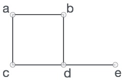
Formally, a graph is a pair of sets (V, E), where V is the set of vertices and E is the set of edges, connecting the pairs of vertices. Take a look at the following graph −
|
Fig 13 - Example
In the above graph,
V = {a, b, c, d, e}
E = {ab, ac, bd, cd, de}
Mathematical graphs can be represented in data structure. We can represent a graph using an array of vertices and a two-dimensional array of edges. Before we proceed further, let's familiarize ourselves with some important terms −
- Vertex − Each node of the graph is represented as a vertex. In the following example, the labeled circle represents vertices. Thus, A to G are vertices. We can represent them using an array as shown in the following image. Here A can be identified by index 0. B can be identified using index 1 and so on.
- Edge − Edge represents a path between two vertices or a line between two vertices. In the following example, the lines from A to B, B to C, and so on represents edges. We can use a two-dimensional array to represent an array as shown in the following image. Here AB can be represented as 1 at row 0, column 1, BC as 1 at row 1, column 2 and so on, keeping other combinations as 0.
- Adjacency − Two node or vertices are adjacent if they are connected to each other through an edge. In the following example, B is adjacent to A, C is adjacent to B, and so on.
- Path − Path represents a sequence of edges between the two vertices. In the following example, ABCD represents a path from A to D.
|
Fig 14 - Path
Following are basic primary operations of a Graph −
- Add Vertex − Adds a vertex to the graph.
- Add Edge − Adds an edge between the two vertices of the graph.
- Display Vertex − Displays a vertex of the graph.
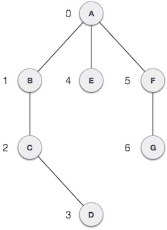
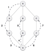
Depth First Search (DFS) algorithm traverses a graph in a depthward motion and uses a stack to remember to get the next vertex to start a search, when a dead end occurs in any iteration.
|
Fig 15 - DFS
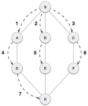
As in the example given above, DFS algorithm traverses from S to A to D to G to E to B first, then to F and lastly to C. It employs the following rules.
- Rule 1 − Visit the adjacent unvisited vertex. Mark it as visited. Display it. Push it in a stack.
- Rule 2 − If no adjacent vertex is found, pop up a vertex from the stack. (It will pop up all the vertices from the stack, which do not have adjacent vertices.)
- Rule 3 − Repeat Rule 1 and Rule 2 until the stack is empty.
Step | Traversal | Description |
1 |
| Initialize the stack. |
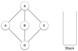
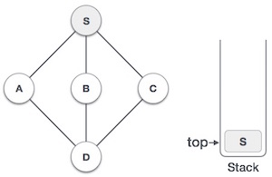
2 |
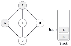
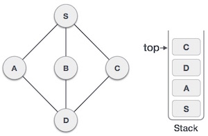
| Mark S as visited and put it onto the stack. Explore any unvisited adjacent node from S. We have three nodes and we can pick any of them. For this example, we shall take the node in an alphabetical order. |
3 |
| Mark A as visited and put it onto the stack. Explore any unvisited adjacent node from A. Both S and D are adjacent to A but we are concerned for unvisited nodes only. |
4 |
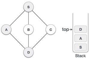
| Visit D and mark it as visited and put onto the stack. Here, we have B and C nodes, which are adjacent to D and both are unvisited. However, we shall again choose in an alphabetical order. |
5 |
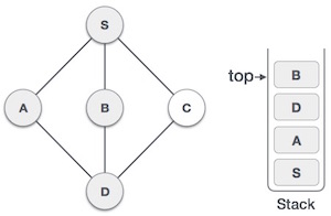
| We choose B, mark it as visited and put onto the stack. Here B does not have any unvisited adjacent node. So, we pop B from the stack. |
6 |
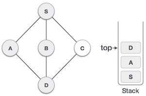
| We check the stack top for return to the previous node and check if it has any unvisited nodes. Here, we find D to be on the top of the stack. |
7 |
| Only unvisited adjacent node is from D is C now. So we visit C, mark it as visited and put it onto the stack. |
As C does not have any unvisited adjacent node so we keep popping the stack until we find a node that has an unvisited adjacent node. In this case, there's none and we keep popping until the stack is empty.
We shall not see the implementation of Depth First Traversal (or Depth First Search) in C programming language. For our reference purpose, we shall follow our example and take this as our graph model −
|
Fig 16 - Example
#include <stdio.h>
#include <stdlib.h>
#include <stdbool.h>
#define MAX 5
struct Vertex {
char label;
bool visited;
};
//stack variables
int stack[MAX];
int top = -1;
//graph variables
//array of vertices
struct Vertex* lstVertices[MAX];
//adjacency matrix
int adjMatrix[MAX][MAX];
//vertex count
int vertexCount = 0;
//stack functions
void push(int item) {
stack[++top] = item;
}
int pop() {
return stack[top--];
}
int peek() {
return stack[top];
}
bool isStackEmpty() {
return top == -1;
}
//graph functions
//add vertex to the vertex list
void addVertex(char label) {
struct Vertex* vertex = (struct Vertex*) malloc(sizeof(struct Vertex));
vertex->label = label;
vertex->visited = false;
lstVertices[vertexCount++] = vertex;
}
//add edge to edge array
void addEdge(int start,int end) {
adjMatrix[start][end] = 1;
adjMatrix[end][start] = 1;
}
//display the vertex
void displayVertex(int vertexIndex) {
printf("%c ",lstVertices[vertexIndex]->label);
}
//get the adjacent unvisited vertex
int getAdjUnvisitedVertex(int vertexIndex) {
int i;
for(i = 0; i < vertexCount; i++) {
if(adjMatrix[vertexIndex][i] == 1 && lstVertices[i]->visited == false) {
return i;
}
}
return -1;
}
void depthFirstSearch() {
int i;
//mark first node as visited
lstVertices[0]->visited = true;
//display the vertex
displayVertex(0);
//push vertex index in stack
push(0);
while(!isStackEmpty()) {
//get the unvisited vertex of vertex which is at top of the stack
int unvisitedVertex = getAdjUnvisitedVertex(peek());
//no adjacent vertex found
if(unvisitedVertex == -1) {
pop();
} else {
lstVertices[unvisitedVertex]->visited = true;
displayVertex(unvisitedVertex);
push(unvisitedVertex);
}
}
//stack is empty, search is complete, reset the visited flag
for(i = 0;i < vertexCount;i++) {
lstVertices[i]->visited = false;
}
}
int main() {
int i, j;
for(i = 0; i < MAX; i++) // set adjacency {
for(j = 0; j < MAX; j++) // matrix to 0
adjMatrix[i][j] = 0;
}
addVertex('S'); // 0
addVertex('A'); // 1
addVertex('B'); // 2
addVertex('C'); // 3
addVertex('D'); // 4
addEdge(0, 1); // S - A
addEdge(0, 2); // S - B
addEdge(0, 3); // S - C
addEdge(1, 4); // A - D
addEdge(2, 4); // B - D
addEdge(3, 4); // C - D
printf("Depth First Search: ")
depthFirstSearch();
return 0;
}
If we compile and run the above program, it will produce the following result −
Depth First Search: S A D B C
Breadth First Search (BFS) algorithm traverses a graph in a breadthward motion and uses a queue to remember to get the next vertex to start a search, when a dead end occurs in any iteration.
|
Fig 17 – BF Traversal
As in the example given above, BFS algorithm traverses from A to B to E to F first then to C and G lastly to D. It employs the following rules.
- Rule 1 − Visit the adjacent unvisited vertex. Mark it as visited. Display it. Insert it in a queue.
- Rule 2 − If no adjacent vertex is found, remove the first vertex from the queue.
- Rule 3 − Repeat Rule 1 and Rule 2 until the queue is empty.
Step | Traversal | Description |
1 |
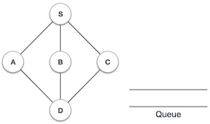
| Initialize the queue. |
2 |
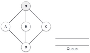
| We start from visiting S (starting node), and mark it as visited. |
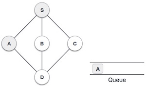
3 |
| We then see an unvisited adjacent node from S. In this example, we have three nodes but alphabetically we choose A, mark it as visited and enqueue it. |
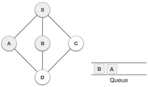
4 |
| Next, the unvisited adjacent node from S is B. We mark it as visited and enqueue it. |
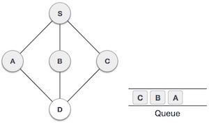
5 |
| Next, the unvisited adjacent node from S is C. We mark it as visited and enqueue it. |
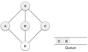
6 |
| Now, S is left with no unvisited adjacent nodes. So, we dequeue and find A. |
7 |
| From A we have D as unvisited adjacent node. We mark it as visited and enqueue it. |
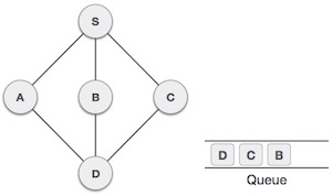
At this stage, we are left with no unmarked (unvisited) nodes. But as per the algorithm we keep on dequeuing in order to get all unvisited nodes. When the queue gets emptied, the program is over.
We shall not see the implementation of Breadth First Traversal (or Breadth First Search) in C programming language. For our reference purpose, we shall follow our example and take this as our graph model −
|
Fig 18 - Example
#include <stdio.h>
#include <stdlib.h>
#include <stdbool.h>
#define MAX 5
struct Vertex {
char label;
bool visited;
};
//queue variables
int queue[MAX];
int rear = -1;
int front = 0;
int queueItemCount = 0;
//graph variables
//array of vertices
struct Vertex* lstVertices[MAX];
//adjacency matrix
int adjMatrix[MAX][MAX];
//vertex count
int vertexCount = 0;
//queue functions
void insert(int data) {
queue[++rear] = data;
queueItemCount++;
}
int removeData() {
queueItemCount--;
return queue[front++];
}
bool isQueueEmpty() {
return queueItemCount == 0;
}
//graph functions
//add vertex to the vertex list
void addVertex(char label) {
struct Vertex* vertex = (struct Vertex*) malloc(sizeof(struct Vertex));
vertex->label = label;
vertex->visited = false;
lstVertices[vertexCount++] = vertex;
}
//add edge to edge array
void addEdge(int start,int end) {
adjMatrix[start][end] = 1;
adjMatrix[end][start] = 1;
}
//display the vertex
void displayVertex(int vertexIndex) {
printf("%c ",lstVertices[vertexIndex]->label);
}
//get the adjacent unvisited vertex
int getAdjUnvisitedVertex(int vertexIndex) {
int i;
for(i = 0; i<vertexCount; i++) {
if(adjMatrix[vertexIndex][i] == 1 && lstVertices[i]->visited == false)
return i;
}
return -1;
}
void breadthFirstSearch() {
int i;
//mark first node as visited
lstVertices[0]->visited = true;
//display the vertex
displayVertex(0);
//insert vertex index in queue
insert(0);
int unvisitedVertex;
while(!isQueueEmpty()) {
//get the unvisited vertex of vertex which is at front of the queue
int tempVertex = removeData();
//no adjacent vertex found
while((unvisitedVertex = getAdjUnvisitedVertex(tempVertex)) != -1) {
lstVertices[unvisitedVertex]->visited = true;
displayVertex(unvisitedVertex);
insert(unvisitedVertex);
}
}
//queue is empty, search is complete, reset the visited flag
for(i = 0;i<vertexCount;i++) {
lstVertices[i]->visited = false;
}
}
int main() {
int i, j;
for(i = 0; i<MAX; i++) // set adjacency {
for(j = 0; j<MAX; j++) // matrix to 0
adjMatrix[i][j] = 0;
}
addVertex('S'); // 0
addVertex('A'); // 1
addVertex('B'); // 2
addVertex('C'); // 3
addVertex('D'); // 4
addEdge(0, 1); // S - A
addEdge(0, 2); // S - B
addEdge(0, 3); // S - C
addEdge(1, 4); // A - D
addEdge(2, 4); // B - D
addEdge(3, 4); // C - D
printf("\nBreadth First Search: ");
breadthFirstSearch();
return 0;
}
If we compile and run the above program, it will produce the following result −
Breadth First Search: S A B C D
Consider a relation R on a set S satisfying the following properties:
- R is reflexive, i.e., xRx for every x ∈ S.
- R is antisymmetric, i.e., if xRy and yRx, then x = y.
- R is transitive, i.e., xRy and yRz, then xRz.
Then R is called a partial order relation, and the set S together with partial order is called a partially order set or POSET and is denoted by (S, ≤).
- The set N of natural numbers form a poset under the relation '≤' because firstly x ≤ x, secondly, if x ≤ y and y ≤ x, then we have x = y and lastly if x ≤ y and y ≤ z, it implies x ≤ z for all x, y, z ∈ N.
- The set N of natural numbers under divisibility i.e., 'x divides y' forms a poset because x/x for every x ∈ N. Also if x/y and y/x, we have x = y. Again if x/y, y/z we have x/z, for every x, y, z ∈ N.
- Consider a set S = {1, 2} and power set of S is P(S). The relation of set inclusion ⊆ is a partial order. Since, for any sets A, B, C in P (S), firstly we have A ⊆ A, secondly, if A ⊆B and B⊆A, then we have A = B. Lastly, if A ⊆B and B ⊆C,then A⊆C. Hence, (P(S), ⊆) is a poset.
- Maximal Element: An element a ∈ A is called a maximal element of A if there is no element in c in A such that a ≤ c.
- Minimal Element: An element b ∈ A is called a minimal element of A if there is no element in c in A such that c ≤ b.
Note: There can be more than one maximal or more than one minimal element.
Example: Determine all the maximal and minimal elements of the poset whose Hasse diagram is shown in fig:
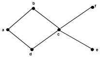
Solution: The maximal elements are b and f.
The minimal elements are d and e.
Consider an ordered set A. Two elements a and b of set A are called comparable if
a ≤ b or b ≤ a
R R
Consider an ordered set A. Two elements a and b of set A are called non-comparable if neither a ≤ b nor b ≤ a.
Example: Consider A = {1, 2, 3, 5, 6, 10, 15, 30} is ordered by divisibility. Determine all the comparable and non-comparable pairs of elements of A.
Solution: The comparable pairs of elements of A are:
{1, 2}, {1, 3}, {1, 5}, {1, 6}, {1, 10}, {1, 15}, {1, 30}
{2, 6}, {2, 10}, {2, 30}
{3, 6}, {3, 15}, {3, 30}
{5, 10}, {5, 15}, {5, 30}
{6, 30}, {10, 30}, {15, 30}
The non-comparable pair of elements of A are:
{2, 3}, {2, 5}, {2, 15}
{3, 5}, {3, 10}, {5, 6}, {6, 10}, {6, 15}, {10, 15}
Consider an ordered set A. The set A is called linearly ordered set or totally ordered set, if every pair of elements in A is comparable.
Example: The set of positive integers I+ with the usual order ≤ is a linearly ordered set.
The topological sorting for a directed acyclic graph is the linear ordering of vertices. For every edge U-V of a directed graph, the vertex u will come before vertex v in the ordering.
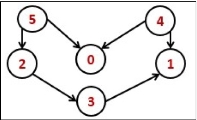
Fig 18 – Topological sorting
As we know that the source vertex will come after the destination vertex, so we need to use a stack to store previous elements. After completing all nodes, we can simply display them from the stack.
Input:
0 0 0 0 0 0
0 0 0 0 0 0
0 0 0 1 0 0
0 1 0 0 0 0
1 1 0 0 0 0
1 0 1 0 0 0
Output:
Nodes after topological sorted order: 5 4 2 3 1 0
topoSort(u, visited, stack)
Input − The start vertex u, An array to keep track of which node is visited or not. A stack to store nodes.
Output − Sorting the vertices in topological sequence in the stack.
Begin
mark u as visited
for all vertices v which is adjacent with u, do
if v is not visited, then
topoSort(c, visited, stack)
done
push u into a stack
End
performTopologicalSorting(Graph)
Input − The given directed acyclic graph.
Output − Sequence of nodes.
Begin
initially mark all nodes as unvisited
for all nodes v of the graph, do
if v is not visited, then
topoSort(i, visited, stack)
done
pop and print all elements from the stack
End.
#include<iostream>
#include<stack>
#define NODE 6
using namespace std;
int graph[NODE][NODE] = {
{0, 0, 0, 0, 0, 0},
{0, 0, 0, 0, 0, 0},
{0, 0, 0, 1, 0, 0},
{0, 1, 0, 0, 0, 0},
{1, 1, 0, 0, 0, 0},
{1, 0, 1, 0, 0, 0}
};
void topoSort(int u, bool visited[], stack<int>&stk) {
visited[u] = true; //set as the node v is visited
for(int v = 0; v<NODE; v++) {
if(graph[u][v]) { //for allvertices v adjacent to u
if(!visited[v])
topoSort(v, visited, stk);
}
}
stk.push(u); //push starting vertex into the stack
}
void performTopologicalSort() {
stack<int> stk;
bool vis[NODE];
for(int i = 0; i<NODE; i++)
vis[i] = false; //initially all nodes are unvisited
for(int i = 0; i<NODE; i++)
if(!vis[i]) //when node is not visited
topoSort(i, vis, stk);
while(!stk.empty()) {
cout << stk.top() << " ";
stk.pop();
}
}
main() {
cout << "Nodes after topological sorted order: ";
performTopologicalSort();
}
Nodes after topological sorted order: 5 4 2 3 1 0
Key takeaway
A graph is a pictorial representation of a set of objects where some pairs of objects are connected by links. The interconnected objects are represented by points termed as vertices, and the links that connect the vertices are called edges.
- Hashing is the process of mapping large amount of data item to smaller table with the help of hashing function.
- Hashing is also known as Hashing Algorithm or Message Digest Function.
- It is a technique to convert a range of key values into a range of indexes of an array.
- It is used to facilitate the next level searching method when compared with the linear or binary search.
- Hashing allows to update and retrieve any data entry in a constant time O(1).
- Constant time O(1) means the operation does not depend on the size of the data.
- Hashing is used with a database to enable items to be retrieved more quickly.
- It is used in the encryption and decryption of digital signatures.
- A fixed process converts a key to a hash key is known as a Hash Function.
- This function takes a key and maps it to a value of a certain length which is called a Hash value or Hash.
- Hash value represents the original string of characters, but it is normally smaller than the original.
- It transfers the digital signature and then both hash value and signature are sent to the receiver. Receiver uses the same hash function to generate the hash value and then compares it to that received with the message.
- If the hash values are same, the message is transmitted without errors.
- Hash table or hash map is a data structure used to store key-value pairs.
- It is a collection of items stored to make it easy to find them later.
- It uses a hash function to compute an index into an array of buckets or slots from which the desired value can be found.
- It is an array of list where each list is known as bucket.
- It contains value based on the key.
- Hash table is used to implement the map interface and extends Dictionary class.
- Hash table is synchronized and contains only unique elements.
|
- The above figure shows the hash table with the size of n = 10. Each position of the hash table is called as Slot. In the above hash table, there are n slots in the table, names = {0, 1, 2, 3, 4, 5, 6, 7, 8, 9}. Slot 0, slot 1, slot 2 and so on. Hash table contains no items, so every slot is empty.
- As we know the mapping between an item and the slot where item belongs in the hash table is called the hash function. The hash function takes any item in the collection and returns an integer in the range of slot names between 0 to n-1.
- Suppose we have integer items {26, 70, 18, 31, 54, 93}. One common method of determining a hash key is the division method of hashing and the formula is :
Hash Key = Key Value % Number of Slots in the Table
- Division method or reminder method takes an item and divides it by the table size and returns the remainder as its hash value.
Data Item | Value % No. of Slots | Hash Value |
26 | 26 % 10 = 6 | 6 |
70 | 70 % 10 = 0 | 0 |
18 | 18 % 10 = 8 | 8 |
31 | 31 % 10 = 1 | 1 |
54 | 54 % 10 = 4 | 4 |
93 | 93 % 10 = 3 | 3 |
|
- After computing the hash values, we can insert each item into the hash table at the designated position as shown in the above figure. In the hash table, 6 of the 10 slots are occupied, it is referred to as the load factor and denoted by, λ = No. of items / table size. For example , λ = 6/10.
- It is easy to search for an item using hash function where it computes the slot name for the item and then checks the hash table to see if it is present.
- Constant amount of time O(1) is required to compute the hash value and index of the hash table at that location.
- Take the above example, if we insert next item 40 in our collection, it would have a hash value of 0 (40 % 10 = 0). But 70 also had a hash value of 0, it becomes a problem. This problem is called as Collision or Clash. Collision creates a problem for hashing technique.
- Linear probing is used for resolving the collisions in hash table, data structures for maintaining a collection of key-value pairs.
- Linear probing was invented by Gene Amdahl, Elaine M. McGraw and Arthur Samuel in 1954 and analyzed by Donald Knuth in 1963.
- It is a component of open addressing scheme for using a hash table to solve the dictionary problem.
- The simplest method is called Linear Probing. Formula to compute linear probing is:
P = (1 + P) % (MOD) Table_size
For example,
|
If we insert next item 40 in our collection, it would have a hash value of 0 (40 % 10 = 0). But 70 also had a hash value of 0, it becomes a problem.
Linear probing solves this problem:
P = H(40)
44 % 10 = 0
Position 0 is occupied by 70. so we look elsewhere for a position to store 40.
Using Linear Probing:
P= (P + 1) % table-size
0 + 1 % 10 = 1
But, position 1 is occupied by 31, so we look elsewhere for a position to store 40.
Using linear probing, we try next position : 1 + 1 % 10 = 2
Position 2 is empty, so 40 is inserted there.
|
Hash Table is a data structure which stores data in an associative manner. In a hash table, data is stored in an array format, where each data value has its own unique index value. Access of data becomes very fast if we know the index of the desired data.
Thus, it becomes a data structure in which insertion and search operations are very fast irrespective of the size of the data. Hash Table uses an array as a storage medium and uses hash technique to generate an index where an element is to be inserted or is to be located from.
Hashing is a technique to convert a range of key values into a range of indexes of an array. We're going to use modulo operator to get a range of key values. Consider an example of hash table of size 20, and the following items are to be stored. Item are in the (key,value) format.
|
Fig 19 – Hash function
- (1,20)
- (2,70)
- (42,80)
- (4,25)
- (12,44)
- (14,32)
- (17,11)
- (13,78)
- (37,98)
Sr.No. | Key | Hash | Array Index |
1 | 1 | 1 % 20 = 1 | 1 |
2 | 2 | 2 % 20 = 2 | 2 |
3 | 42 | 42 % 20 = 2 | 2 |
4 | 4 | 4 % 20 = 4 | 4 |
5 | 12 | 12 % 20 = 12 | 12 |
6 | 14 | 14 % 20 = 14 | 14 |
7 | 17 | 17 % 20 = 17 | 17 |
8 | 13 | 13 % 20 = 13 | 13 |
9 | 37 | 37 % 20 = 17 | 17 |
As we can see, it may happen that the hashing technique is used to create an already used index of the array. In such a case, we can search the next empty location in the array by looking into the next cell until we find an empty cell. This technique is called linear probing.
Sr.No. | Key | Hash | Array Index | After Linear Probing, Array Index |
1 | 1 | 1 % 20 = 1 | 1 | 1 |
2 | 2 | 2 % 20 = 2 | 2 | 2 |
3 | 42 | 42 % 20 = 2 | 2 | 3 |
4 | 4 | 4 % 20 = 4 | 4 | 4 |
5 | 12 | 12 % 20 = 12 | 12 | 12 |
6 | 14 | 14 % 20 = 14 | 14 | 14 |
7 | 17 | 17 % 20 = 17 | 17 | 17 |
8 | 13 | 13 % 20 = 13 | 13 | 13 |
9 | 37 | 37 % 20 = 17 | 17 | 18 |
Following are the basic primary operations of a hash table.
- Search − Searches an element in a hash table.
- Insert − inserts an element in a hash table.
- delete − Deletes an element from a hash table.
Define a data item having some data and key, based on which the search is to be conducted in a hash table.
struct DataItem {
int data;
int key;
};
Define a hashing method to compute the hash code of the key of the data item.
int hashCode(int key){
return key % SIZE;
}
Whenever an element is to be searched, compute the hash code of the key passed and locate the element using that hash code as index in the array. Use linear probing to get the element ahead if the element is not found at the computed hash code.
struct DataItem *search(int key) {
//get the hash
int hashIndex = hashCode(key);
//move in array until an empty
while(hashArray[hashIndex] != NULL) {
if(hashArray[hashIndex]->key == key)
return hashArray[hashIndex];
//go to next cell
++hashIndex;
//wrap around the table
hashIndex %= SIZE;
}
return NULL;
}
Whenever an element is to be inserted, compute the hash code of the key passed and locate the index using that hash code as an index in the array. Use linear probing for empty location, if an element is found at the computed hash code.
void insert(int key,int data) {
struct DataItem *item = (struct DataItem*) malloc(sizeof(struct DataItem));
item->data = data;
item->key = key;
//get the hash
int hashIndex = hashCode(key);
//move in array until an empty or deleted cell
while(hashArray[hashIndex] != NULL && hashArray[hashIndex]->key != -1) {
//go to next cell
++hashIndex;
//wrap around the table
hashIndex %= SIZE;
}
hashArray[hashIndex] = item;
}
Whenever an element is to be deleted, compute the hash code of the key passed and locate the index using that hash code as an index in the array. Use linear probing to get the element ahead if an element is not found at the computed hash code. When found, store a dummy item there to keep the performance of the hash table intact.
struct DataItem* delete(struct DataItem* item) {
int key = item->key;
//get the hash
int hashIndex = hashCode(key);
//move in array until an empty
while(hashArray[hashIndex] !=NULL) {
if(hashArray[hashIndex]->key == key) {
struct DataItem* temp = hashArray[hashIndex];
//assign a dummy item at deleted position
hashArray[hashIndex] = dummyItem;
return temp;
}
//go to next cell
++hashIndex;
//wrap around the table
hashIndex %= SIZE;
}
return NULL;
}
Hash Table is a data structure which stores data in an associative manner. In hash table, the data is stored in an array format where each data value has its own unique index value. Access of data becomes very fast, if we know the index of the desired data.
#include <stdio.h>
#include <string.h>
#include <stdlib.h>
#include <stdbool.h>
#define SIZE 20
struct DataItem {
int data;
int key;
};
struct DataItem* hashArray[SIZE];
struct DataItem* dummyItem;
struct DataItem* item;
int hashCode(int key) {
return key % SIZE;
}
struct DataItem *search(int key) {
//get the hash
int hashIndex = hashCode(key);
//move in array until an empty
while(hashArray[hashIndex] != NULL) {
if(hashArray[hashIndex]->key == key)
return hashArray[hashIndex];
//go to next cell
++hashIndex;
//wrap around the table
hashIndex %= SIZE;
}
return NULL;
}
void insert(int key,int data) {
struct DataItem *item = (struct DataItem*) malloc(sizeof(struct DataItem));
item->data = data;
item->key = key;
//get the hash
int hashIndex = hashCode(key);
//move in array until an empty or deleted cell
while(hashArray[hashIndex] != NULL && hashArray[hashIndex]->key != -1) {
//go to next cell
++hashIndex;
//wrap around the table
hashIndex %= SIZE;
}
hashArray[hashIndex] = item;
}
struct DataItem* delete(struct DataItem* item) {
int key = item->key;
//get the hash
int hashIndex = hashCode(key);
//move in array until an empty
while(hashArray[hashIndex] != NULL) {
if(hashArray[hashIndex]->key == key) {
struct DataItem* temp = hashArray[hashIndex];
//assign a dummy item at deleted position
hashArray[hashIndex] = dummyItem;
return temp;
}
//go to next cell
++hashIndex;
//wrap around the table
hashIndex %= SIZE;
}
return NULL;
}
void display() {
int i = 0;
for(i = 0; i<SIZE; i++) {
if(hashArray[i] != NULL)
printf(" (%d,%d)",hashArray[i]->key,hashArray[i]->data);
else
printf(" ~~ ");
}
printf("\n");
}
int main() {
dummyItem = (struct DataItem*) malloc(sizeof(struct DataItem));
dummyItem->data = -1;
dummyItem->key = -1;
insert(1, 20);
insert(2, 70);
insert(42, 80);
insert(4, 25);
insert(12, 44);
insert(14, 32);
insert(17, 11);
insert(13, 78);
insert(37, 97);
display();
item = search(37);
if(item != NULL) {
printf("Element found: %d\n", item->data);
} else {
printf("Element not found\n");
}
delete(item);
item = search(37);
if(item != NULL) {
printf("Element found: %d\n", item->data);
} else {
printf("Element not found\n");
}
}
If we compile and run the above program, it will produce the following result −
~~ (1,20) (2,70) (42,80) (4,25) ~~ ~~ ~~ ~~ ~~ ~~ ~~ (12,44) (13,78) (14,32) ~~ ~~ (17,11) (37,97) ~~
Element found: 97
Element not found
Collision Resolution Techniques
- In this, the hash function is used to compute the index of the array.
- The hash value is used to store the key in the hash table, as an index.
- The hash function can return the same hash value for two or more keys.
- When two or more keys are given the same hash value, it is called a collision. To handle this collision, we use collision resolution techniques.
Collision resolution techniques
There are two types of collision resolution techniques.
- Separate chaining (open hashing)
- Open addressing (closed hashing)
In this technique, a linked list is created from the slot in which collision has occurred, after which the new key is inserted into the linked list. This linked list of slots looks like a chain, so it is called separate chaining. It is used more when we do not know how many keys to insert or delete.
Time complexity
- Its worst-case complexity for searching is o(n).
- Its worst-case complexity for deletion is o(n).
Advantages of separate chaining
- It is easy to implement.
- The hash table never fills full, so we can add more elements to the chain.
- It is less sensitive to the function of the hashing.
Disadvantages of separate chaining
- In this, cache performance of chaining is not good.
- The memory wastage is too much in this method.
- It requires more space for element links.
Open addressing is collision-resolution method that is used to control the collision in the hashing table. There is no key stored outside of the hash table. Therefore, the size of the hash table is always greater than or equal to the number of keys. It is also called closed hashing.
The following techniques are used in open addressing:
- Linear probing
- Quadratic probing
- Double hashing
In this, when the collision occurs, we perform a linear probe for the next slot, and this probing is performed until an empty slot is found. In linear probing, the worst time to search for an element is O(table size). The linear probing gives the best performance of the cache but its problem is clustering. The main advantage of this technique is that it can be easily calculated.
Disadvantages of linear probing
- The main problem is clustering.
- It takes too much time to find an empty slot.
In this, when the collision occurs, we probe for i2th slot in ith iteration, and this probing is performed until an empty slot is found. The cache performance in quadratic probing is lower than the linear probing. Quadratic probing also reduces the problem of clustering.
In this, you use another hash function, and probe for (i * hash 2(x)) in the ith iteration. It takes longer to determine two hash functions. The double probing gives the very poor the cache performance, but there has no clustering problem in it.
Hashing with Chaining in Data Structure
In this section we will see what is the hashing with chaining. The Chaining is one collision resolution technique. We cannot avoid collision, but we can try to reduce the collision, and try to store multiple elements for same hash value.
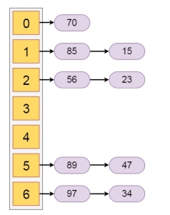
this technique suppose our hash function h(x) ranging from 0 to 6. So for more than 7 elements, there must be some elements, that will be places inside the same room. For that we will create a list to store them accordingly. In each time we will add at the beginning of the list to perform insertion in O(1) time
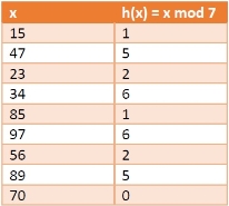
Let us see the following example to get better idea. If we have some elements like {15, 47, 23, 34, 85, 97, 65, 89, 70}. And our hash function is h(x) = x mod 7.
The hash values will be
The Hashing with chaining will be like −
|
Key takeaway
- Hashing is the process of mapping large amount of data item to smaller table with the help of hashing function.
- Hashing is also known as Hashing Algorithm or Message Digest Function.
- It is a technique to convert a range of key values into a range of indexes of an array.
- It is used to facilitate the next level searching method when compared with the linear or binary search.
- Hashing allows to update and retrieve any data entry in a constant time O(1).
- Constant time O(1) means the operation does not depend on the size of the data.
- Hashing is used with a database to enable items to be retrieved more quickly.It is used in the encryption and decryption of digital signatures.
Reference
1 Data structure & algorithm analysis in C by Mark Allen Weiss published by Pearson Education (LPE)
2 Introduction to Data structure in C by A.N. Kathie published by Pearson Education (LPE)
