UNIT-1
Probability Theory, Random Variable & Process
Let A and B be two events of a sample space Sand let  . Then conditional probability of the event A, given B, denoted by
 is defined by –

Theorem: If the events A and B defined on a sample space S of a random experiment are independent, then

Example1: A factory has two machines A and B making 60% and 40% respectively of the total production. Machine A produces 3% defective items, and B produces 5% defective items. Find the probability that a given defective part came from A.
SOLUTION: We consider the following events:
A: Selected item comes from A.
B: Selected item comes from B.
D: Selected item is defective.
We are looking for  . We know:
Now,
So we need
|
Since, D is the union of the mutually exclusive events  and
and  (the entire sample space is the union of the mutually exclusive events A and B)
|
Key Takeaways:
If the events A and B defined on a sample space S of a random experiment are independent, then

Conditional probabilities arise naturally in the investigation of experiments where an outcome of trial affect the outcomes of the subsequent trials.
We try to calculate the probability of the second event (event B) given that the first event (event A) has already happened. If the probability of the event changes when we take the first event into consideration, we can safely say that the probability of event B is dependent of the occurrence of event A.
For example
- Drawing a second ace from a deck given we got the first ace
- Finding the probability of having a disease given you were tested positive
- Finding the probability of liking Harry Potter given we know the person likes fiction
Here there are 2 events:
- Event A is the probability of the event we are trying to calculate.
- Event B is the condition that we know or the event that has happened.
Hence we write the conditional probability as P ( A/B) , the probability of the occurrence of event A given that B has already happened.
P(A/B) = P( A and B) / P(B) = Probability of occurrence of both A and B / Probability of B
Suppose you draw two cards from a deck and you win if you get a jack followed by an ace (without replacement). What is the probability of winning, given we know that you got a jack in the first turn?
Let event A be getting a jack in the first turn
Let event B be getting an ace in the second turn.
We need to find P(B/A)
P(A) = 4/52
P(B) = 4/51 {no replacement}
P(A and B) = 4/52*4/51= 0.006
P(B/A) = P( A and B)/ P(A) = 0.006/0.077 = 0.078
Here we are determining the probabilities when we know some conditions instead of calculating random probabilities
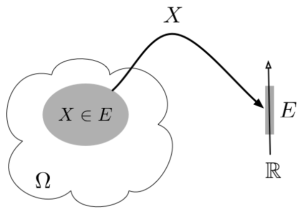
A random variable (RV) X is a function from the sample space Ω to the real numbers X:Ω→R Assuming E⊂RE⊂R we denote the event {ω∈Ω:X(ω)∈E}⊂Ω by {X∈E} or just X∈E.
|
Fig.1: Random variable
The probability distribution of a discrete random variable is a list of probabilities associated with each of its possible values. It is also sometimes called the probability function or the probability mass function.
Suppose a random variable X may take k different values, with the probability that X = xi defined to be P(X = xi) = pi. The probabilities pi must satisfy the following:
1: 0 < pi < 1 for each i
2: p1 + p2 + ... + pk = 1.
Example
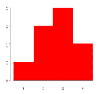
Suppose a variable X can take values 1,2,3, or 4. The probabilities associated with each outcome are described by the following table:
Outcome 1 2 3 4 Probability 0.1 0.3 0.4 0.2
|
The probability that X is equal to 2 or 3 is the sum of the two probabilities:
P(X = 2 or X = 3) = P(X = 2) + P(X = 3) = 0.3 + 0.4 = 0.7.
Similarly, the probability that X is greater than 1 is equal to 1 - P(X = 1)
= 1 - 0.1 = 0.9,
A continuous random variable is as function that maps the sample space of a random experiment to an interval in the real value space. A random variable is called continuous if there is an underlying function f(x) such that
P(p q) =
q) =  dx
dx
f(x) is non-negative function called the probability density function. From the rules of probability
P(- < X < ∞) =
  dx =1
dx =1
Probability density function
Probability density function is defined by following formula:
P(a≤X≤b)=
Where −
- [a,b][a,b] = Interval in which x lies.
- P(a≤X≤b)= probability that some value x lies within this interval.
- dx = b-a
f(x) = {1/24, 0, for 0 x
x  24
24
0 otherwise
Calculate the probability that clock stops between 2 pm and 2:45 pm.
Solution:
We have found the value of the following:
P(14  14.45 )
=  dx
dx
= 1/24 (0.45)
= 0.01875
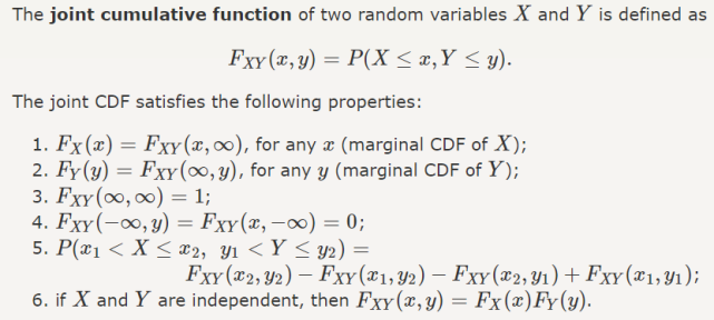
Joint CDF & PDF
|
The mean (or average), mu, of the sample is the first moment:
You will also see this notation sometimes
In R, the mean() function returns the average of a vector. |
A continuous random variable XX is said to have a Uniform distribution over the interval [a,b], shown as X ∼ Uniform (a,b), if its PDF is given by
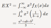
To find the variance, we can find EX2 using LOTUS:
|
The Rayleigh distribution is a continuous probability distribution named after the English Lord Rayleigh. The distribution is widely used:
- In communications theory, to model multiple paths of dense scattered signals reaching a receiver.
- In the physical sciences to model wind speed, wave heights and sound/light radiation.
- In engineering, to measure the lifetime of an object, where the lifetime depends on the object’s age. For example: resistors, transformers, and capacitors in aircraft radar sets.1
- In medical imaging science, to model noise variance in magnetic resonance imaging.
The Rayleigh distribution is a special case of the Weibull distribution with a scale parameter of 2. When a Rayleigh is set with a shape parameter (σ) of 1, it is equal to a chi square distribution with 2 degrees of freedom.
The notation X Rayleigh(σ) means that the random variable X has a Rayleigh distribution with shape parameter σ. The probability density function (X > 0) is:
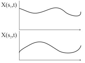
A useful extension of the idea of random variables is the random process. While the random variable X is defined as a univariate function X(s) where s is the outcome of a random experiment, the random process is a bivariate function X(s, t) where s is the outcome of a random experiment and t is an index variable such as time.
Examples of random processes are the voltages in a circuit over time, light intensity over location. The random process, for two outcomes s1 and s2 can be plotted as
|
Fig.2: Random Process
Two Ways to View a Random Process
• A random process can be viewed as a function X(t, ω) of two variables, time t ∈ T and the outcome of the underlying random experiment ω ∈ Ω
◦ For fixed t, X(t, ω) is a random variable over Ω
◦ For fixed ω, X(t, ω) is a deterministic function of t, called a sample function
|
Fig.3: Random Process
A random process is said to be discrete time if T is a countably infinite set, e.g., ◦ N = {0, 1, 2, . . .} ◦ Z = {. . . , −2, −1, 0, +1, +2, . . .}
• In this case the process is denoted by Xn, for n ∈ N , a countably infinite set, and is simply an infinite sequence of random variables
• A sample function for a discrete time process is called a sample sequence or sample path
• A discrete-time process can comprise discrete, continuous, or mixed r.v.s
Example
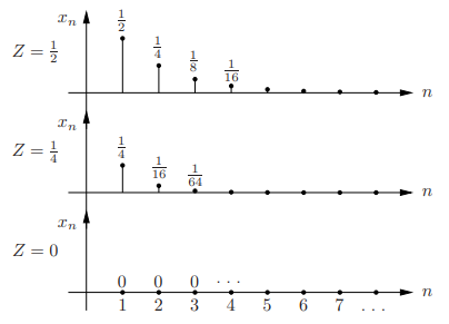
• Let Z ∼ U[0, 1], and define the discrete time process Xn = Z n for n ≥ 1
• Sample paths:
|
Fig.4: Sample paths
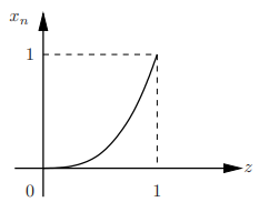
First-order pdf of the process: For each n, Xn = Z n is a r.v.; the sequence of pdfs of Xn is called the first-order pdf of the process
|
Fig.5: First-order pdf of the process
Since Xn is a differentiable function of the continuous r.v. Z, we can find its pdf as f
fXn (x) = 1/( nx(n−1)/n) = 1/n x(1/n)−1) , 0 ≤ x ≤ 1
Key Takeaways:
- A random process can be viewed as a function X(t, ω) of two variables, time t ∈ T and the outcome of the underlying random experiment ω ∈ Ω
- A sample function for a discrete time process is called a sample sequence or sample path.
A random process is said to be ergodic if the time averages of the process tend to the appropriate ensemble averages. This definition implies that with probability 1, any ensemble average of {X(t)} can be determined from a single sample function of {X(t)}. Clearly, for a process to be ergodic, it has to necessarily be stationary. But not all stationary processes are ergodic.
A process in which ensemble average (at a given time) of an observable quantity <O>E=∫O e-βE dp dq / ∫ e-βE dpdq
remains equal to the time average
<O>t= lim t →∞ (1/t) ∫0t O(t) dt, is an ergodic process.
Autocorrelation are commonly used for measuring the similarity of signals especially for “pattern recognition” and for “signal detection.”
Example: Autocorrelation used to extract radar signals to improve sensitivity. Makes use of radar signals being periodic so the signal is a pulse train (parameters: amplitude, pulse width and interval between pulses).
Autocorrelation measurements have become a standard method for pulse characterization of ultrafast laser pulses
References:
- Information theory and coding by Giridhar
- Information theory and coding by JS Chitode


