UNIT - 5
Frequency Domain Techniques
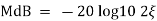
Resonant Peak (Mr): The maximum value of magnitude is known as Resonant peak. The relative stability of the system can be determined by Mr. The larger the value of Mr the undesirable is the transient response.
Resonant Frequency (Wr): The frequency at which magnitude has maximum value.
Bandwidth: The band of frequencies lying between -3db points.
Cut-off frequency –The frequency at which the magnitude is 3db below its zero frequency.
Cut-off Rate – It is the slope of the log magnitude curve near the cut off frequency.
| |
|
|
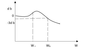
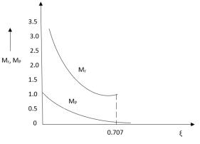
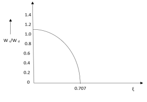
Fig 1 Frequency Domain Specification
The transfer function of second order system is shown as C(S)/R(S) = W2n / S2 + 2ξWnS + W2n - - (1) ξ = Ramping factor Wn = Undamped natural frequency for frequency response let S = jw C(jw) / R(jw) = W2n / (jw)2 + 2 ξWn(jw) + W2n
Let U = W/Wn above equation becomes T(jw) = W2n / 1 – U2 + j2 ξU so, | T(jw) | = M = 1/√(1 – u2)2 + (2ξU)2 - - (2) T(jw) = φ = -tan-1[ 2ξu/(1-u2)] - - (3) For sinusoidal input the output response for the system is given by C(t) = 1/√(1-u2)2 + (2ξu)2Sin[wt - tan-1 2ξu/1-u2] - - (4) The frequency where M has the peak value is known as Resonant frequency Wn. This frequency is given as (from eqn (2)). dM/du|u=ur = Wr = Wn√(1-2ξ2) - - (5) from equation(2) the maximum value of magnitude is known as Resonant peak. Mr = 1/2ξ√1-ξ2 - - (6) The phase angle at resonant frequency is given as Φr = - tan-1 [√1-2ξ2/ ξ] - - (7) As we already know for step response of second order system the value of damped frequency and peak overshoot are given as Wd = Wn√1-ξ2 - - (8) Mp = e- πξ2|√1-ξ2 - - (9) |
The comparison of Mr and Mp is shown in figure(1). The two performance indices are correlated as both are functions of the damping factor ξ only. When subjected to step input the system with given value of Mr of its frequency response will exhibit a corresponding value of Mp.
Similarly the correlation of Wr and Wd is shown in fig(2) for the given input step response [ from eqn(5) & eqn(8) ]
Wr/Wd = √(1- 2ξ2)/(1-ξ2)
Mp = Peak overshoot of step response
Mr = Resonant Peak of frequency response
Wr = Resonant frequency of Frequency response
Wd = Damping frequency of oscillation of step response.
From fig(1) it is clear that for ξ> 1/2, value of Mr does not exists.
Key takeaway
- Mr and Mp are correlated as both are functions of the damping factor ξ only
- When subjected to step input the system with given value of Mr of its frequency response will exhibit a corresponding value of Mp.
In polar plot any point gives the magnitude phase of the transfer function in bode we split magnitude and  plot.
plot.
Advantages
- By looking at bode plot we can write the transfer function of system
Q. G(S) = 1. substitute S = j G(j M =
Magnitude varies with ‘w’ but phase is constant. MdB = +20 log10
Decade frequency :- W present = 10 Then
0.01 40 0.1 20 1 0 (shows pole at origin) 0 -20 10 -40 100 -60 Slope = (20db/decade) |
|


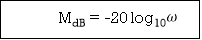


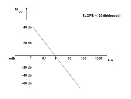
Fig 2 MAGNITUDE PLOT
|
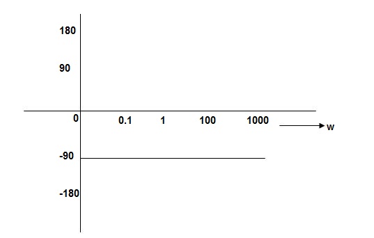
Fig 3 PHASE PLOT
Example-1 G(S) = 
Sol: G(j M = MdB = +20 log MdB = -40 log10
0.01 80 0.1 40 1 0 (pole at origin) 10 -40 100 -80 Slope = 40dbdecade |


Example-2 G(S) = S
Sol: M= W
MdB = 20 log10
0.01 -40 0.1 -20 1 0 10 20 100 90 1000 60 |
|


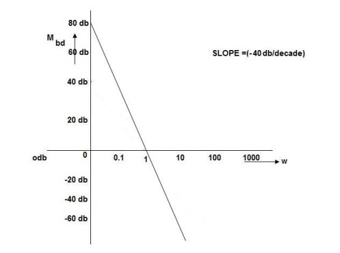
Fig 4 Bode Plot G(S) = S
Example-3 G(S) = S2
Sol: M= MdB = 20 log10
W MdB 0.01 -80 0.1 -40 1 0 10 40 100 80
|


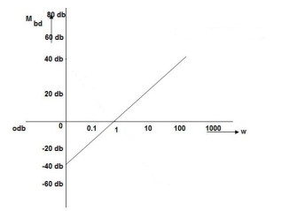
Fig 5 Magnitude Plot G(S) = S2
Example-6 G(S) = 
Sol: : G(j M = MdB = 20 log10 K-20 log10
K=1 K=10
=-20 log10 0.01 40 60 0.1 20 40 1 0 20 10 -20 0 100 -40 -20
|


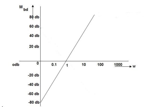
Fig 6 Bode Plot G(S) = 
|
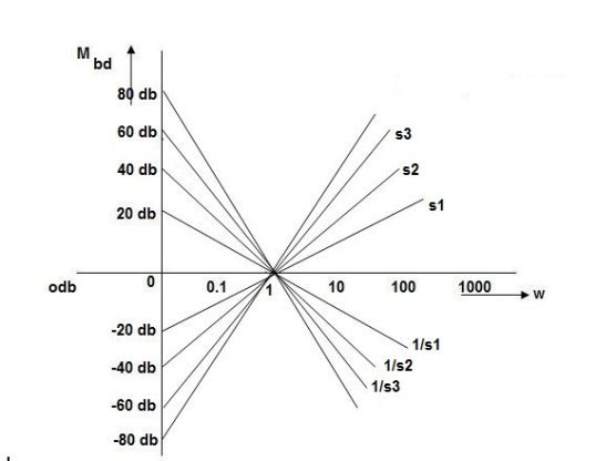
Fig 7 All bode plots in one plot
|
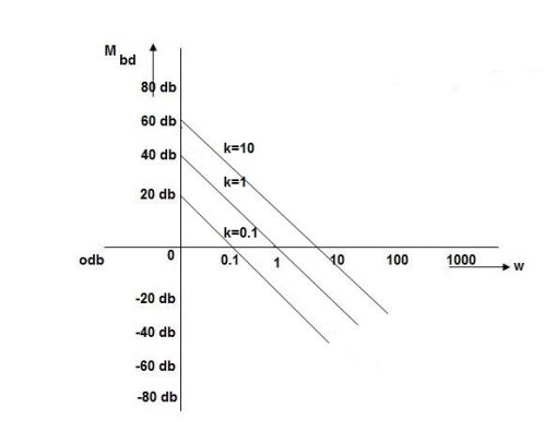
Fig 8 Variation in K shifts magnitude plot by +20db
As we vary K  then plot shift by 20 log10K i.e adding a d.c. to a.c. quantity
Approximation of Bode Plot:
If poles and zeros are not located at origin G(S) = TF = M = MdB = -20 log10 (
Approximation: MdB = -20 log10 MdB = -20 log10 Approximation: MdB= 0dB, At a point both meet so equal i.e a time will come hence both approx become equal -20 log10
At this frequency both the cases are equal MdB = -20 log10 Now for MdB = -20 log10 = -20 log10 = -10 log102 MdB = 10 |
|


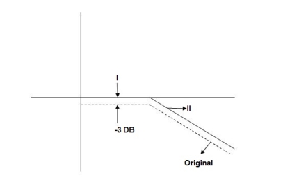
Fig 9 Approximation in bode plot
When we increase the value of  in app 2 and decrease the
  of app 1 so a RT comes when both cases are equal and hence for that value of
  where both app are equal gives max. error we found above and is equal to 3dB. At corner frequency we have max error of -3dB
Key takeaway
For every zero, the slope changes by -20db/decade. For every pole the slope changes by +20db/decade.
It gives the frequency response as well as comments on the stability and the relative stability of the system.
Nyquist Stability Criteria:
The Nyquist criteria is a semi graphical method that determines stability of CL system investigating the properties of the frequency domain plot (Polar plot), the Nyquist plot of the OLTF G(S) H(S) is represented as L(S)
L(S) = G(S)H(S)
Specially the Nyquist plot of L(S) is a plot drawn by substituting S=jw and varying the value of w as per in polar plot. In polar plot we take one sided frequency response ( 0 - ∞) in Nyquist plot we will vary the frequency in entire range possible from ( -∞ to 0 ) and (0 to ∞ )
Nyquist Criteria also gives: -
(1). In addition to providing the absolute stability like other plots, the Nyquist criteria also gives information on the relative stability of a stable system and the degree of instability of an unstable system.
(2). It also gives indications on how the system stability can be improved.
(3). The Nyquist plot of G(S) H(S) is the polar plot of G(S) H(S) drawn with wider range of frequency ( -∞ to ∞ ) and along the Nyquist path.
(4). The Nyquist plot of G(S) H(S) gives information on frequency domain characteristics such as B.W, gain margin and phase margin.
Construction of Nyquist Plot
Encircled: A point or region in a complex function phase i.e. S-plane is said to be encircled by a closed path if it is found inside the path.
Assumption: -
|
|
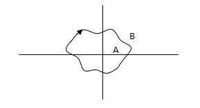
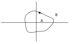
Fig 10 Encirclement
In this example point A is encircled by the closed path Y. Since, A is inside the closed path point B is not encircled by y. it is outside the path. Furthermore, when the closed path Y, has a direction assign to it, encirclement, if made can be in the clockwise direction or in the anti-clockwise direction.
Point A is encircled by Y by anticlockwise direction. We can say that the region inside the path is encircled in the prescribed direction and the region outside the path is not encircled.
Enclosed: -
A point or region is said to be enclosed by a closed path if it is encircled in the counter clockwise direction, or the point or region lies to the left of the path (always), when the path is traveling in the prescribed direction.
The concept of enclosure is particularly useful, if only a portion of a closed path is shown.
In this example the shaded region are
|
|
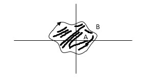
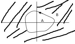
Fig 11 Enclosure
Considered to be enclosed by the closed path Y. In other words, point A is enclosed by Y in fig a. but is not enclosed by Y in fig b. and for point B it is vice versa.
No of encirclements and enclosures:
For A line is cut once For B line is cut twice
|
|

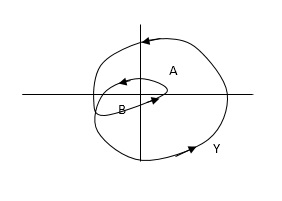
Fig 12 Encirclement and Enclosure with example
As it’s overlapping but 2 times in Same direction
When a point is encircled by a closed path Y, a no. N can be assigned to the no. of times it is encircled. The magnitude of N can be determined by drawing an arrow around the closed path Y.
Taking an arbitrary point S, and moving around in clockwise direction and anti-clockwise direction respectively. We are getting a direction.
The path followed by S1 gives us the direction and this path which covers the total number of revolution travelled by this point S1 is N or the net angle is ‘ 2 π N ’.
For B = 2 = N for A = 1 = N
In this eg. point A is encircled ones (or 2 π radians) by function Y and point B is encircled twice (or 4 π radians) all in clockwise direction.
In diagram b again A and B are encircled but in counter clockwise direction thus for this diagram A is enclosed one’s and B is enclosed twice.
By definition M is +ve for anticlockwise(direction) encirclement and –ve for clockwise encirclement.
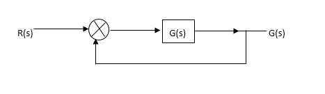
OLTF G(S) = (S + Z1)(S + Z2)/(S + P1)(S + P2) H(S) = 1 - - (1)
|
Fig 13 Unity feedback control system |
CLTF G(S)/1 + G(S) CE = 1 + G(S) = 1 + (S + Z1)(S + Z2)/(S + P1)(S + P2) CE = (S + P1)(S + P2) + (S + Z1)(S + Z2)/ (S + P1)(S + P2) - - (2) |
Key takeaway:
# OLTF poles is equal to CE poles. CE = (S + Z’1)( S + Z’2)/( S + P1)( S + P2) - - (3) CLTF = G(S) –(1) / 1 + G(S) –(3) = (S + Z1)( S + Z2) / (S + Z’1)( S + Z’2) - - (4) |
The frequency at which the bode plot culls the 0db axis is called as Gain Cross Over Frequency.
|
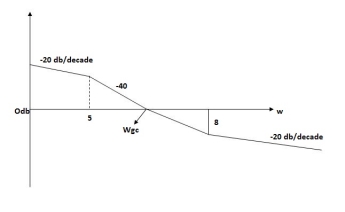
Fig 14 Gain cross over frequency
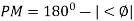
- Phase Cross Over Frequency
The Frequency at which the phase plot culls the -1800 axis.
|
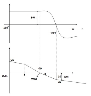
Fig 15 Phase Margin and Gain Margin
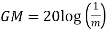
GM=MdB= -20 log [ G (jw)]
|


1) When gain cross over frequency is smaller then phase curves over frequency the system is stable and vice versa.
Key takeaway:
- More the difference b/WPC and WGC core is the stability of system
- If GM is below 0dB axis than take ilb +ve and stable. if GM above 0dB axis , that is take -ve
- GM= ODB - 20 log M
- The IM should also lie above -1800 for making the system (i.e. pm=+ve
- For a stable system GM and PM should be -ve
- GM and PM both should be +ve more the value of GM and PM more the system is stable.
- If Wpc and Wgc are in same line Wpc= Wgc than system is marginally stable . as we get GM=0dB.
Nyquist diagram
Consider a contour, which covers the entire right half of S-plane.
|
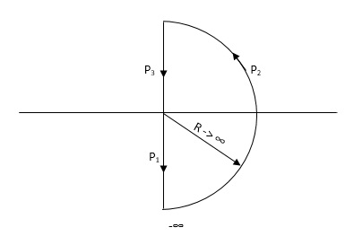
Fig 16 Contour For Right half of S-plane
P1 W(0 - ∞) P2 RejR ∞ ϴ - π/2 to 0 to + π/2 P3 W(∞ to 0 ) |
If each and every point along the boundary of contour is mapped in q(S) where q(S) is 1+G(S)H(S)[CE]. The CE is drawn in S-domain. Now, as the CE: q(s) = 1 + G(S)H(S) contour is drawn into S-plane.
This q(S) contour may encircle the origin. Thus, the number of encirclements of q(S) contour with respect to origin is given by
N = Z – P
Where: Z1P zeros and poles of q(S)[CE]
N Total no of encirclement of origin
- Z1P Zeros and poles of CE in the right half of S-plane
Note: for the CL system to be stable Z=0 always.
Important:Open loop System(stable) :- When OL system is stable P=0 i.e. no of poles on right half
N = Z – P
If P = 0
N = Z
- Now for CL system to be stable Z = 0
- N = 0
- i.e. q(s) contour should not encircle the origin.
Open loop system(unstable) :-Let P = 1 i.e. one OL pole is located in right half of S-plane i.e. OLTF is unstable.
As N = Z – P
N = Z – 1
For CL system to be stable the only criteria is (Z=0) i.e.
N = -1
which means q(S) contour should encircle the origin one’s in CW direction.
Key takeaway:
(1). When OL system is unstable then corresponding CL will be stable only when q(S) contour will encircle origin in CW direction.
(2). The no of encirclements should be equal to no of open loop poles located in right half of S-plane.
NOTE The no of encirclements(N) can also be calculated by using G(S) contour (instead of q(S) contour) but the reference is -1+j0 instead of 0+j0 i.e. the no of encirclements should be considered w.r.t -1+j0 and not with the origin.
Explanation Mapping
q(S) = 1 + G(S)
G(S) is always given to us, so we can relate G(S) with q(S).
G(S) = q(S) – 1
But q(S) can be drawn by adding 1 real part to the q(S).
|
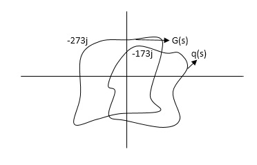
Fig 17 Mapping
G(S) given then q(S) shift to right side.
Q1. For the transfer function below plot the Nyquist plot and also comment on stability?
G(S) = 1/S+1
Sol:- N = Z – P ( No pole of right half of S plane P = 0 ) P = 0, N = Z NYQUIST PATH :- P1 = W – (0 to - ∞) P2 = ϴ( - π/2 to 0 to π/2 ) P3 = W(+∞ to 0) |
|
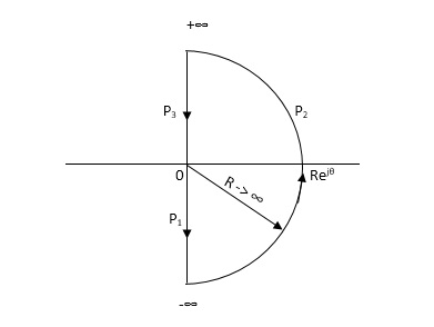
Fig 18 Nyquist path
Substituting S = jw G(jw) = 1/jw + 1 M = 1/√1+W2 Φ = -tan-1(W/I) for P1 :- W(0 to -∞) W M φ 0 1 0 -1 1/√2 +450 -∞ 0 +900 Path P2 :- W = Rejϴ R ∞ϴ -π/2 to 0 to π/2 G(jw) = 1/1+jw = 1/1+j(Rejϴ) (neglecting 1 as R ∞) M = 1/Rejϴ = 1/R e-jϴ M = 0 e-jϴ = 0 Path P3 :- W = -∞ to 0 M = 1/√1+W2 , φ = -tan-1(W/I)
W M φ ∞ 0 -900 1 1/√2 -450 0 1 00 The Nyquist Plot is shown in fig 13 |
|
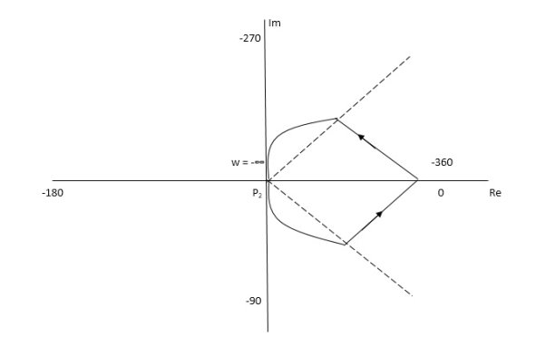
Fig 19 Nyquist Plot G(S) = 1/S+1
From plot we can see that -1 is not encircled so, N = 0
But N = Z, Z = 0
So, system is stable.
Q.2. for the transfer function below plot the Nyquist Plot and comment on stability G(S) = 1/(S + 4)(S + 5)
Soln :- N = Z – P , P = 0, No pole on right half of S-plane
N = Z
NYQUIST PATH P1 = W(0 to -∞) P2 = ϴ(-π/2 to 0 to +π/2) P3 = W(∞ to 0) |
|

Fig 20 Nyquist Path
Path P1 W(0 to -∞) M = 1/√42 + w2 √52 + w2 Φ = -tan-1(W/4) – tan-1(W/5) W M Φ 0 1/20 00 -1 0.047 25.350 -∞ 0 +1800 Path P3 will be the mirror image across the real axis. Path P2 :ϴ(-π/2 to 0 to +π/2) S = Rejϴ G(S) = 1/(Rejϴ + 4)( Rejϴ + 5) R∞ = 1/ R2e2jϴ = 0.e-j2ϴ = 0 The plot is shown in fig 15. From plot N=0, Z=0, system stable. |
|
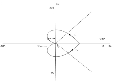
Fig 21 Nyquist Plot G(S) = 1/(S + 4)(S + 5)
Q.3. For the given transfer function, plot the Nyquist plot and comment on stability G(S) = k/S2(S + 10)?
Soln: As the poles exists at origin. So, first time we do not include poles in Nyquist plot. Then check the stability for second case we include the poles at origin in Nyquist path. Then again check the stability.
PART – 1 : Not including poles at origin in the Nyquist Path.
|
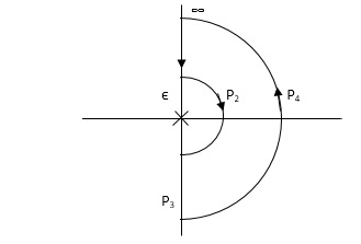
Fig 22 Nyquist Path
P1 W(∞ Ɛ) where Ɛ 0 P2 S = Ɛejϴ ϴ(+π/2 to 0 to -π/2) P3 W = -Ɛ to -∞ P4 S = Rejϴ, R ∞, ϴ = -π/2 to 0 to +π/2 For P1 M = 1/w.w√102 + w2 = 1/w2√102 + w2 Φ = -1800 – tan-1(w/10) W M Φ ∞ 0 -3 π/2 Ɛ ∞ -1800 Path P3 will be mirror image of P1 about Real axis. G(Ɛ ejϴ) = 1/( Ɛ ejϴ)2(Ɛ ejϴ + 10) Ɛ 0, ϴ = π/2 to 0 to -π/2 = 1/ Ɛ2 e2jϴ(Ɛ ejϴ + 10) = ∞. e-j2ϴ [ -2ϴ = -π to 0 to +π ] Path P2 will be formed by rotating through -π to 0 to +π Path P4 S = Rejϴ R ∞ ϴ = -π/2 to 0 to +π/2 G(Rejϴ) = 1/ (Rejϴ)2(10 + Rejϴ) = 0 N = Z – P No poles on right half of S plane so, P = 0 N = Z – 0 |
|
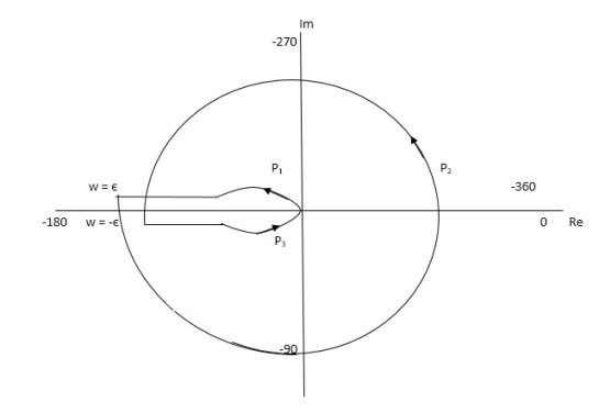
Fig 23 Nyquist Plot for G(S) = k/S2(S + 10)
But from plot shown in fig 22. it is clear that number of encirclements in Anticlockwise direction. So,
N = 2 N = Z – P 2 = Z – 0 Z = 2 Hence, system unstable. PART 2 Including poles at origin in the Nyquist Path |
|
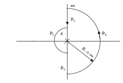
Fig 24 Nyquist Path
P1 W(∞ to Ɛ) Ɛ 0 P2 S = Ɛejϴ Ɛ 0 ϴ(+π/2 to +π to +3π/2) P3 W(-Ɛ to -∞) Ɛ 0 P4 S = Rejϴ, R ∞, ϴ(3π/2 to 2π to +5π/2) M = 1/W2√102 + W2 , φ = - π – tan-1(W/10) P1 W(∞ to Ɛ) W M φ ∞ 0 -3 π/2 Ɛ ∞ -1800 P3( mirror image of P1) P2 S = Ɛejϴ G(Ɛejϴ) = 1/ Ɛ2e2jϴ(10 + Ɛejϴ) Ɛ 0 G(Ɛejϴ) = 1/ Ɛ2e2jϴ(10) = ∞. e-j2ϴϴ(π/2 to π to 3π/2) -2ϴ = (-π to -2π to -3π) P4 = 0 |
|
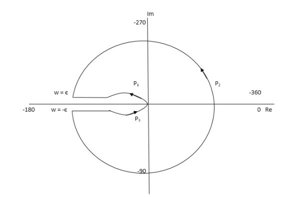
Fig 25 Nyquist Plot G(S) = k/S2(S + 10)
The plot is shown in fig 25. from the plot it is clear that there is no encirclement of -1 in Nyquist path. (N = 0). But the two poles at origin lies to the right half of S-plane in Nyquist path.(P = 2)[see path P2]
N = Z – P
0 = Z – 2
Z = 2
Hence, system is unstable.
Path P2 will be formed by rotating through -π to -2π to -3π
NOTE: The sign convention for angles is shown
|
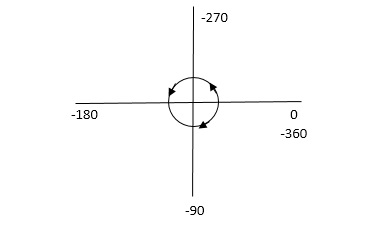
Fig 26 Sign for Angle Directions
Angles are considered –ve for anticlockwise directions and +ve for clockwise directions.
Bode Plot
Que. G(S) = 
Sol: TF = 
M = 
MdB = -20 log10 ( at T=2
 MdB
MdB
1 -20 log10
10 -20 log10
100 -20 log10
 MdB
MdB  =
= =
= 
0.1 -20 log10 = 1.73
  10-3
10-3
0.1 -20 log10 = -0.1703
0.5 -20 log10 = -3dB
1 -20 log10 = -6.98
10 -20 log10 = -26.03
100 -20 log10 = -46.02
|
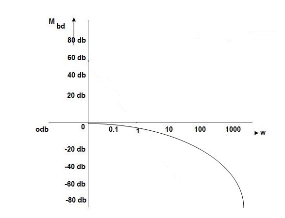
Fig 27 Magnitude Plot with approximation
Without approximation
For second order system TF = TF = = = = M= MdB= Case 1 MdB= 20 log10 Case 2 MdB = -20 log10 = -20 log10 = -20 log10
MdB = -20 log10 = -40 log10 Case 3 . when case 1 is equal to case 2 -40 log10
|


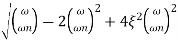


The natural frequency is our corner frequency
|
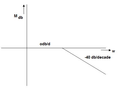
Fig 28 Magnitude Plot
Max error at  i.e at corner frequency
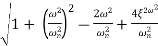
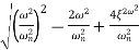
MdB = -20 log10 For MdB = -20 log10
Completely the error depends upon the value of The maximum error will be MdB = -20 log10 M = -20 log10
|


 is resonant frequency and at this frequency we are getting the maximum error so the magnitude will be
M = - = Mr = MdB = -20 log10 MdB = -20 log10
Mr = |


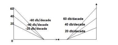
Type of system | Initial slope | Intersection |
0 | 0 dB/decade | Parallel to 0 axis |
1 | -20 dB/decade | =K1 |
2 | -40 dB/decade | =K1/2 |
3 | -60 dB/decade | =K1/3 |
. | . | 1 |
. | . | 1 |
. | . | 1 |
N | -20N dB/decade | =K1/N |
effect can be understood by plotting few bode plots as shown below
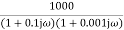
Q.1 sketch the bode plot for transfer function
G(S) = 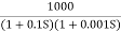
- Replace S = j

|


- For phase plot
For phase plot
100 -900 200 -9.450 300 -104.80 400 -110.360 500 -115.420 600 -120.00 700 -124.170 800 -127.940 900 -131.350 1000 -134.420 The plot is shown in figure below |
|
|


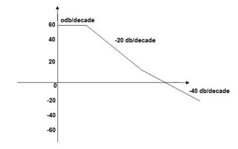
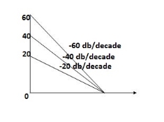
Fig 29 Magnitude Plot for G(S) = 
Q.2 For the given transfer function determine
G(S) = 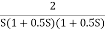
Gain cross over frequency phase cross over frequency phase mergence and gain margin
Initial slope = 1
N = 1 , (K)1/N = 2
K = 2
Corner frequency
 1 =
1 =  = 2 (slope -20 dB/decade
 2 =
2 =  = 20 (slope -40 dB/decade

2. phase
 = tan-1
 - tan-1 0.5
  - tan-1 0.05
 = 900- tan-1 0.5
  - tan-1 0.05
1 -119.430 5 -172.230 10 -195.250 15 -209.270 20 -219.30 25 -226.760 30 -232.490 35 -236.980 40 -240.570 45 -243.490 50 -245.910
Finding M = 4 =
Let X3 (6.25 X1 = 2.46 X2 = -399.9 X3 = -6.50 For x1 = 2.46
for phase margin PM = 1800 -
= -164.50 PM = 1800 - 164.50 = 15.50 For phase cross over frequency (
-1800 = -900 – tan-1 (0.5 -900 – tan-1 (0.5 Taking than on both sides Tan 900 = tan-1 Let tan-1 0.5
1 =0.5
|


the plot is shown i figure below
|
|
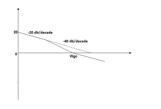
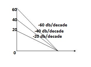
Fig 30 Magnitude Plot G(S) = 
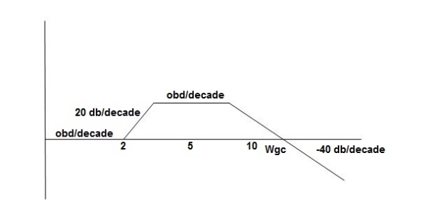
Q3. For the given transfer function
G(S) = Plot the rode plot find PM and GM T1 = 0.5 Zero so, slope (20 dB/decade) T2 = 0.2 Pole , so slope (-20 dB/decade) T3 = 0.1 = T4 = 0.1
|


- Initial slope 0 dB/decade till
 1 = 2 rad/sec
 - From
 1 to
1 to 2 (i.e. 2 rad /sec to 5 rad/sec) slope will be 20 dB/decade
 - From
 2 to
2 to  3 the slope will be 0 dB/decade (20 + (-20))
 - From
 3 ,
3 , 4 the slope will be -40 dB/decade (0-20-20)
Phase plot
500 -177.30 1000 -178.60 1500 -179.10 2000 -179.40 2500 -179.50 3000 -179.530 3500 -179.60 GM = 00 PM = 61.460 The plot is shown in figure below |
|
|


|
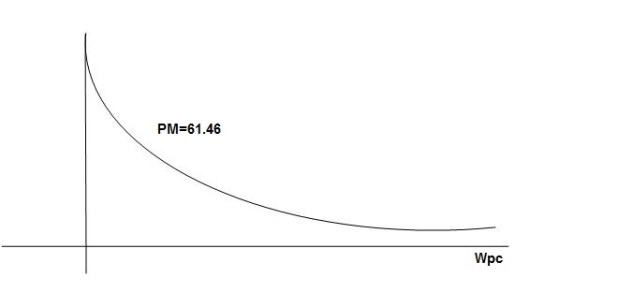
Fig 31 Magnitude and phase Plot for G(S) = 
Q 4. For the given transfer function plot the bode plot (magnitude plot) G(S) = 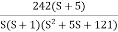
Sol: Given transfer function
G(S) = Converting above transfer function to standard from G(S) = = |

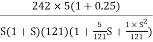
As type 1 system , so initial slope will be -20 dB/decade
- Final slope will be -60 dB/decade as order of system decides the final slope
- Corner frequency
- T1 =
 ,
,  11= 5 (zero)
 - T2 = 1 ,
 2 = 1 (pole)
- T1 =
- Initial slope will cut zero dB axis at
- (K)1/N = 10
- i.e
 = 10
= 10
- finding
 n and
n and 
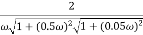
T(S) = T(S)= Comparing with standard second order system equation S2+2
M = -20 log 2 = +6.5 dB 2. As K = 10, so whole plot will shift by 20 log 10 10 = 20 dB The plot is shown in figure below |
|
|


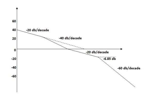
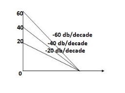
Fig 32 Magnitude Plot for G(S) = 
Q5. For the given plot determine the transfer function
|
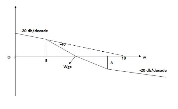
Fig 33 Magnitude Plot
Sol: From figure above, we can conclude that
- Initial slope = -20 dB/decade so type -1
- Initial slope all 0 dB axis at
 = 10 so
K1/N N = 1
(K)1/N = 10.
3. corner frequency
 1 =
1 =  = 0.2 rad/sec
 2 =
2 =  = 0.125 rad/sec
- At
 = 5 the slope becomes -40 dB/decade, so there is a pole at
  = 5 as
slope changes from -20 dB/decade to -40 dB/decade
- At
 = 8 the slope changes from -40 dB/decade to -20 dB/decade hence is a zero at
  = 8 (-40+(+20) = 20)
Hence transfer function is T(S) = 
Effect of addition of zeros
- Stability of system increases.
- The settling time decreases.
- The gain margin increases.
- The system becomes less oscillatory.
Effect of Addition of Poles:
- The system becomes oscillatory.
- The stability of system decreases.
- The settling time increases.
- The range of k reduces.
References:
1. “Control System Engineering”, Norman S. Nise,John willey and Sons, 6th Edition, 2015.
2. “Control System Engineering”,I.J. Nagrath and M. Gopal,New age International publication, 5th Edition, 2014.
3. “Modern Control Engineering”, Katsuhiko Ogata,Prentice Hall of India Pvt
Ltd, 5th edition.
4. “Automatic Control System”, Benjamin C. Kuo, Prentice Hall of India Pvt Ltd, Wiley publication, 9th edition


