Unit – II
Correlation Analysis
Correlation is used to describe the linear relationship between two continuous variables (e.g., height and weight). In general, correlation tends to be used when there is no identified response variable. It measures the strength (qualitatively) and direction of the linear relationship between two or more variables.
Definition
“Correlation analysis deals with the association between two or more variables.” —Simpson and Kafka
“Correlation is an analysis of the co-variation between two variables.” —A.M. Tuttle
Importance
Correlation is very important in the field of Psychology and Education as a measure of relationship between test scores and other measures of performance. With the help of correlation, it is possible to have a correct idea of the working capacity of a person. With the help of it, it is also possible to have a knowledge of the various qualities of an individual.
After finding the correlation between the two qualities or different qualities of an individual, it is also possible to provide his vocational guidance. In order to provide educational guidance to a student in selection of his subjects of study, correlation is also helpful and necessary.
Types
Correlation measures the nature and strength of relationship between two variables. Correlation lies between +1 to -1. A correlation of +1 indicates a perfect positive correlation between two variables. A zero correlation indicates that there is no relationship between the variables. A correlation of -1 indicates a perfect negative correlation.
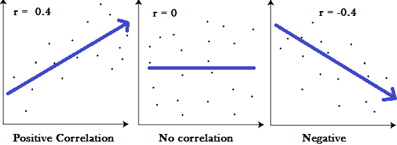
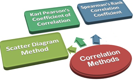
Measures of correlation
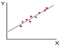
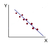
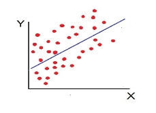
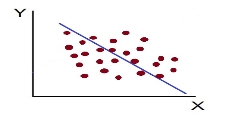
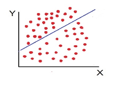
The more the points plotted are scattered over the chart, the lesser is the degree of correlation between the variables. The more the points plotted are closer to the line, the higher is the degree of correlation. The degree of correlation is denoted by “r”.
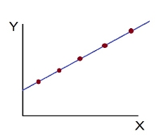
b. Perfect negative correlation (r=-1) – all the points plotted on the straight line falling from left to right
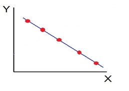
c. High Degree of +Ve Correlation (r= + High): all the points plotted close to the straight line rising from left to right
d. High Degree of –Ve Correlation (r= – High) - all the points plotted close to the straight line falling from left to right.
e. Low degree of +Ve Correlation (r= + Low): all the points are highly scattered to the straight line rising from left to right
f. Low Degree of –Ve Correlation (r= - Low): all the points are highly scattered to the straight line falling from left to right
g. No Correlation (r= 0) – all the points are scattered over the graph and do not show any pattern
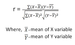
2. Karl Pearson’s Coefficient of Correlation is widely used mathematical method is used to calculate the degree and direction of the relationship between linear related variables. The coefficient of correlation is denoted by “r”.
Direct method
Shortcut method –


The value of the coefficient of correlation (r) always lies between ±1. Such as:
h. r=+1, perfect positive correlation
i. r=-1, perfect negative correlation
j. r=0, no correlation
k.
Example 1 - Compute Pearsons coefficient of correlation between advertisement cost and sales as per the data given below:
Advertisement cost | 39 | 65 | 62 | 90 | 82 | 75 | 25 | 98 | 36 | 78 |
sales | 47 | 53 | 58 | 86 | 62 | 68 | 60 | 91 | 51 | 84 |
Solution
X | Y |
|
|
|
| |
39 | 47 | -26 | 676 | -19 | 361 | 494 |
65 | 53 | 0 | 0 | -13 | 169 | 0 |
62 | 58 | -3 | 9 | -8 | 64 | 24 |
90 | 86 | 25 | 625 | 20 | 400 | 500 |
82 | 62 | 17 | 289 | -4 | 16 | -68 |
75 | 68 | 10 | 100 | 2 | 4 | 20 |
25 | 60 | -40 | 1600 | -6 | 36 | 240 |
98 | 91 | 33 | 1089 | 25 | 625 | 825 |
36 | 51 | -29 | 841 | -15 | 225 | 435 |
78 | 84 | 13 | 169 | 18 | 324 | 234 |
650 | 660 |
| 5398 |
| 2224 | 2704 |
|
|
|
|
|
|
|

r = (2704)/√5398 √2224 = (2704)/(73.2*47.15) = 0.78
Thus Correlation coefficient is positively correlated.
Example 2
Compute correlation coefficient from the following data
Hours of sleep (X) | Test scores (Y) |
8 | 81 |
8 | 80 |
6 | 75 |
5 | 65 |
7 | 91 |
6 | 80 |
X | Y |
|
|
|
| |
8 | 81 | 1.3 | 1.8 | 2.3 | 5.4 | 3.1 |
8 | 80 | 1.3 | 1.8 | 1.3 | 1.8 | 1.8 |
6 | 75 | -0.7 | 0.4 | -3.7 | 13.4 | 2.4 |
5 | 65 | -1.7 | 2.8 | -13.7 | 186.8 | 22.8 |
7 | 91 | 0.3 | 0.1 | 12.3 | 152.1 | 4.1 |
6 | 80 | -0.7 | 0.4 | 1.3 | 1.8 | -0.9 |
40 | 472 |
| 7 |
| 361 | 33 |

X = 40/6 =6.7

Y = 472/6 = 78.7

r = (33)/√7 √361 = (33)/(2.64*19) = 0.66
Thus Correlation coefficient is positively correlated.
Example 3
Calculate coefficient of correlation between X and Y series using Karl pearson shortcut method
X | 14 | 12 | 14 | 16 | 16 | 17 | 16 | 15 |
Y | 13 | 11 | 10 | 15 | 15 | 9 | 14 | 17 |
Let assumed mean for X = 15, assumed mean for Y = 14
X | Y | dx | dx2 | dy | dy2 | dxdy |
14 | 13 | -1.0 | 1.0 | -1.0 | 1.0 | 1.0 |
12 | 11 | -3.0 | 9.0 | -3.0 | 9.0 | 9.0 |
14 | 10 | -1.0 | 1.0 | -4.0 | 16.0 | 4.0 |
16 | 15 | 1.0 | 1.0 | 1.0 | 1.0 | 1.0 |
16 | 15 | 1.0 | 1.0 | 1.0 | 1.0 | 1.0 |
17 | 9 | 2.0 | 4.0 | -5.0 | 25.0 | -10.0 |
16 | 14 | 1 | 1 | 0 | 0 | 0 |
15 | 17 | 0 | 0 | 3 | 9 | 0 |
120 | 104 | 0 | 18 | -8 | 62 | 6 |

 r = 8 *6 – (0)*(-8)
√8*18-(0)2 √8*62 – (-8)2
r = 48/√144*√432 = 0.19
Example 4 - Calculate coefficient of correlation between X and Y series using Karl pearson shortcut method
X | 1800 | 1900 | 2000 | 2100 | 2200 | 2300 | 2400 | 2500 | 2600 |
F | 5 | 5 | 6 | 9 | 7 | 8 | 6 | 8 | 9 |
Solution
Assumed mean of X and Y is 2200, 6
X | Y | dx | dx (i=100) | dx2 | dy | dy2 | dxdy |
1800 | 5 | -400 | -4 | 16 | -1.0 | 1.0 | 4.0 |
1900 | 5 | -300 | -3 | 9 | -1.0 | 1.0 | 3.0 |
2000 | 6 | -200 | -2 | 4 | 0.0 | 0.0 | 0.0 |
2100 | 9 | -100 | -1 | 1 | 3.0 | 9.0 | -3.0 |
2200 | 7 | 0 | 0 | 0 | 1.0 | 1.0 | 0.0 |
2300 | 8 | 100 | 1 | 1 | 2.0 | 4.0 | 2.0 |
2400 | 6 | 200 | 2 | 4 | 0 | 0 | 0.0 |
2500 | 8 | 300 | 3 | 9 | 2 | 4 | 6.0 |
2600 | 9 | 400 | 4 | 16 | 3 | 9 | 12.0 |
|
|
|
|
|
|
|
|
|
|
| 0 | 60 | 9 | 29 | 24 |
Note – we can also proceed dividing x/100
 r = (9)(24) – (0)(9)
√9*60-(0)2 √9*29– (9)2
r = 0.69
Example 5 –
X | 28 | 45 | 40 | 38 | 35 | 33 | 40 | 32 | 36 | 33 |
Y | 23 | 34 | 33 | 34 | 30 | 26 | 28 | 31 | 36 | 35 |
Solution
X | Y |
|
|
|
| |
28 | 23 | -8 | 64 | -8.0 | 64.0 | 64.0 |
45 | 34 | 9 | 81 | 3.0 | 9.0 | 27.0 |
40 | 33 | 4 | 16 | 2.0 | 4.0 | 8.0 |
38 | 34 | 2 | 4 | 3.0 | 9.0 | 6.0 |
35 | 30 | -1 | 1 | -1.0 | 1.0 | 1.0 |
33 | 26 | -3 | 9 | -5.0 | 25.0 | 15.0 |
40 | 28 | 4 | 16 | -3 | 9 | -12.0 |
32 | 31 | -4 | 16 | 0 | 0 | 0.0 |
36 | 36 | 0 | 0 | 5 | 25 | 0.0 |
33 | 35 | -3 | 9 | 4 | 16 | -12 |
360 | 310 | 0 | 216 | 0 | 162 | 97 |

 X = 360/10 = 36
Y = 310/10 = 31

r = 97/(√216 √162 = 0.51
3. Spearman’s Rank Correlation Coefficient - The Spearman’s Rank Correlation Coefficient is the non-parametric statistical measure used to study the strength of association between the two ranked variables. This method is used for ordinal set of numbers, which can be arranged in order.

Where, P = Rank coefficient of correlation
D = Difference of ranks
N = Number of Observations
The Spearman’s Rank Correlation coefficient lies between +1 to -1.
l. +1 indicates perfect association of rank
m. 0 indicates no association between the rank
n. -1 indicates perfect negative association between the ranks
When ranks are not given - Rank by taking the highest value or the lowest value as 1
Equal Ranks or Tie in Ranks – in this case ranks are assigned on an average basis. For ex – if three students score of 5, at 5th, 6th, 7th ranks ach one of them will be assigned a rank of 5 + 6 + 7/3= 6.
If two individual ranked equal at third position, then the rank is calculates as (3+4)/2 = 3.5
Example 1 –
Test 1 | 8 | 7 | 9 | 5 | 1 |
Test 2 | 10 | 8 | 7 | 4 | 5 |
Solution
Here, highest value is taken as 1
Test 1 | Test 2 | Rank T1 | Rank T2 | d | d2 |
8 | 10 | 2 | 1 | 1 | 1 |
7 | 8 | 3 | 2 | 1 | 1 |
9 | 7 | 1 | 3 | -2 | 4 |
5 | 4 | 4 | 5 | -1 | 1 |
1 | 5 | 5 | 4 | 1 | 1 |
|
|
|
|
| 8 |

R = 1 – (6*8)/5(52 – 1) = 0.60
Example 2 -
Calculate Spearman rank-order correlation
English | 56 | 75 | 45 | 71 | 62 | 64 | 58 | 80 | 76 | 61 |
Maths | 66 | 70 | 40 | 60 | 65 | 56 | 59 | 77 | 67 | 63 |
Solution
Rank by taking the highest value or the lowest value as 1.
Here, highest value is taken as 1
English | Maths | Rank (English) | Rank (Math) | d | d2 |
56 | 66 | 9 | 4 | 5 | 25 |
75 | 70 | 3 | 2 | 1 | 1 |
45 | 40 | 10 | 10 | 0 | 0 |
71 | 60 | 4 | 7 | -3 | 9 |
62 | 65 | 6 | 5 | 1 | 1 |
64 | 56 | 5 | 9 | -4 | 16 |
58 | 59 | 8 | 8 | 0 | 0 |
80 | 77 | 1 | 1 | 0 | 0 |
76 | 67 | 2 | 3 | -1 | 1 |
61 | 63 | 7 | 6 | 1 | 1 |
|
|
|
|
| 54 |

 R = 1-(6*54)
10(102-1)
R = 0.67
Therefore this indicates a strong positive relationship between the ranks individuals obtained in the math and English exam.
Example 3 –
Find Spearman's rank correlation coefficient between X and Y for this set of data:
X | 13 | 20 | 22 | 18 | 19 | 11 | 10 | 15 |
Y | 17 | 19 | 23 | 16 | 20 | 10 | 11 | 18 |
Solution
X | Y | Rank X | Rank Y | d | d2 |
13 | 17 | 3 | 4 | -1 | 1 |
20 | 19 | 7 | 6 | 1 | 1 |
22 | 23 | 8 | 8 | 0 | 0 |
18 | 16 | 5 | 3 | 2 | 2 |
19 | 20 | 6 | 7 | -1 | 1 |
11 | 10 | 2 | 1 | 1 | 1 |
10 | 11 | 1 | 2 | -1 | 1 |
15 | 18 | 4 | 5 | -1 | 1 |
|
|
|
|
| 8 |
R =

 R = 1 – 6*8/8(82 – 1) = 1 – 48 = 0.90
504
Example 4 – Calculation of equal ranks or tie ranks
Find Spearman's rank correlation coefficient:
Commerce | 15 | 20 | 28 | 12 | 40 | 60 | 20 | 80 |
Science | 40 | 30 | 50 | 30 | 20 | 10 | 30 | 60 |
Solution
C | S | Rank C | Rank S | d | d2 |
15 | 40 | 2 | 6 | -4 | 16 |
20 | 30 | 3.5 | 4 | -0.5 | 0.25 |
28 | 50 | 5 | 7 | -2 | 4 |
12 | 30 | 1 | 4 | -3 | 9 |
40 | 20 | 6 | 2 | 4 | 16 |
60 | 10 | 7 | 1 | 6 | 36 |
20 | 30 | 3.5 | 4 | -0.5 | 0.25 |
80 | 60 | 8 | 8 | 0 | 0 |
|
|
|
|
| 81.5 |

R = 1 – (6*81.5)/8(82 – 1) = 0.02
Example 5 –
X | 10 | 15 | 11 | 14 | 16 | 20 | 10 | 8 | 7 | 9 |
Y | 16 | 16 | 24 | 18 | 22 | 24 | 14 | 10 | 12 | 14 |
Solution
X | Y | Rank X | Rank Y | d | d2 |
10 | 16 | 6.5 | 5.5 | 1 | 1 |
15 | 16 | 3 | 5.5 | -2.5 | 6.25 |
11 | 24 | 5 | 1.5 | 3.5 | 12.25 |
14 | 18 | 4 | 4 | 0 | 0 |
16 | 22 | 2 | 3 | -1 | 1 |
20 | 24 | 1 | 1.5 | -0.5 | 0.25 |
10 | 14 | 6.5 | 7.5 | -1 | 1 |
8 | 10 | 9 | 10 | -1 | 1 |
7 | 12 | 10 | 9 | 1 | 1 |
9 | 14 | 8 | 7.5 | 0.5 | 0.25 |
|
|
|
|
| 24 |

R = 1 – (6*24)/10(102 – 1) = 0.85
The correlation between X and Y is positive and very high.
Regression analysis is a technique of studying the dependence of one variable called dependent variable, on one or more variable called explanatory variable, with a view to estimate or predict the average value of the dependent variables in terms of the known or fixed values of the independent variables.
Regression analysis includes several variations, such as linear, multiple linear, and nonlinear. The most common models are simple linear and multiple linear.
Nonlinear regression analysis is commonly used for more complicated data sets in which the dependent and independent variables show a nonlinear relationship.
Difference between correlation and Regression.
Correlation | Regression |
‘Correlation’ as the name says it determines the interconnection or a co-relationship between the variables. | ‘Regression’ explains how an independent variable is numerically associated with the dependent variable. |
In Correlation, both the independent and dependent values have no difference. | However, in Regression, both the dependent and independent variable are different. |
The primary objective of Correlation is, to find out a quantitative/numerical value expressing the association between the values. | When it comes to regression, its primary intent is, to reckon the values of a haphazard variable based on the values of the fixed variable. |
Correlation stipulates the degree to which both of the variables can move together. | However, regression specifies the effect of the change in the unit, in the known variable(p) on the evaluated variable (q). |
Correlation helps to constitute the connection between the two variables. | Regression helps in estimating a variable’s value based on another given value. |
Lines of Regression:
Simple linear regression
Simple linear regression is a model that assesses the relationship between a dependent variable and an independent variable.
Y = a + bX + ϵ
Where:
Y – Dependent variable
X – Independent (explanatory) variable
a – Intercept
b – Slope
ϵ – Residual (error)
With the help of simple linear regression model we have the following two regression lines-
1. Regression line of Y on X: This line gives the probable value of Y (Dependent variable) for any given value of X (Independent variable).
Regression line of Y on X : Y – Ẏ = byx (X – Ẋ)
OR : Y = a + bX
2. Regression line of X on Y: This line gives the probable value of X (Dependent variable) for any given value of Y (Independent variable).
Regression line of X on Y : X – Ẋ = bxy (Y – Ẏ)
OR : X = a + bY
Multiple linear regressions.
Multiple linear regression analysis is essentially similar to the simple linear model, with the exception that multiple independent variables are used in the model.
Y = a + bX1 + cX2 + dX3 + ϵ
Where:
Y – Dependent variable
X1, X2, X3 – Independent (explanatory) variables
a – Intercept
b, c, d – Slopes
ϵ – Residual (error)
Example
How to find a linear regression equation
Subject | X | Y |
1 | 43 | 99 |
2 | 21 | 65 |
3 | 25 | 79 |
4 | 42 | 75 |
5 | 57 | 87 |
6 | 59 | 81 |
|
|
|
Solution
Subject | X | Y | Xy | X2 | Y2 |
1 | 43 | 99 | 4257 | 1849 | 9801 |
2 | 21 | 65 | 1365 | 441 | 4225 |
3 | 25 | 79 | 1975 | 625 | 6241 |
4 | 42 | 75 | 3150 | 1764 | 5625 |
5 | 57 | 87 | 4959 | 3249 | 7569 |
6 | 59 | 81 | 4779 | 3481 | 6521 |
Total | 247 | 486 | 20485 | 11409 | 40022 |
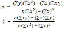
To find a and b, use the following equation
Find a:
((486 × 11,409) – ((247 × 20,485)) / 6 (11,409) – 247*247)
484979 / 7445
=65.14
Find b:
(6(20,485) – (247 × 486)) / (6 (11409) – 247*247)
(122,910 – 120,042) / 68,454 – 2472
2,868 / 7,445
= .385225
y’ = a + bx
y’ = 65.14 + .385225x
Example
Calculate linear regression analysis
students | X | Y |
1 | 95 | 85 |
2 | 85 | 95 |
3 | 80 | 70 |
4 | 70 | 65 |
5 | 60 | 70 |
Solution
students | X | Y | X2 | y2 | Xy |
1 | 95 | 85 | 9025 | 7225 | 8075 |
2 | 85 | 95 | 7225 | 9025 | 8075 |
3 | 80 | 70 | 6400 | 4900 | 5600 |
4 | 70 | 65 | 4900 | 4225 | 4550 |
5 | 60 | 70 | 3600 | 4900 | 4200 |
Total | 390 | 385 | 31150 | 30275 | 30500 |
To find a and b, use the following equation
Find a:
((385 × 31150) – ((390 × 30500)) / 5 (31150) – 152100)
97750 / 3650
=26.78
Find b:
(5(30500) – (390 × 385)) / (5 (31150) – 152100)
2,350 / 3650
= .0.64
y’ = a + bx
y’ = 26.78 + .0.64x
Properties of Regression lines
Key takeaways –
Fitting straight lines
The line of best fit is a line from which the sum of the deviations of various points is zero. This is the best method for obtaining the trend values. It gives a convenient basis for calculating the line of best fit for the time series. It is a mathematical method for measuring trend. Further the sum of the squares of these deviations would be least when compared with other fitting methods. So, this method is known as the Method of Least Squares and satisfies the following conditions:
(i) The sum of the deviations of the actual values of Y and Ŷ (estimated value of Y) is Zero. that is Σ(Y–Ŷ) = 0.
(ii) The sum of squares of the deviations of the actual values of Y and Ŷ (estimated value of Y) is least. that is Σ(Y–Ŷ)2 is least;
Procedure:
(i) The straight line trend is represented by the equation Y = a + bX …(1)
where Y is the actual value, X is time, a, b are constants
(ii) The constants ‘a’ and ‘b’ are estimated by solving the following two normal
Equations ΣY = n a + b ΣX ...(2)
ΣXY = a ΣX + b ΣX2 ...(3)
Where ‘n’ = number of years given in the data.
(iii) By taking the mid-point of the time as the origin, we get ΣX = 0
(iv) When ΣX = 0 , the two normal equations reduces to
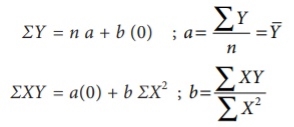
The constant ‘a’ gives the mean of Y and ‘b’ gives the rate of change (slope).
(v) By substituting the values of ‘a’ and ‘b’ in the trend equation (1), we get the Line of Best Fit.
Regression coefficient and their properties:
The quantity “b” in the regression equation is called as the regression coefficient or slope coefficient. Since there are two regression equations, therefore, we have two regression coefficients.
1. Regression Coefficient X on Y, symbolically written as “bxy”
2. Regression Coefficient Y on X, symbolically written as “byx”
Different formula’s used to compute regression coefficients:

Properties of Regression Coefficients:

Estimation of dependent variable:
The estimates of the Y-intercept and slope minimize the sum of the squared residuals, and are called the least squares estimates. Explained above.
Example 1
Find the two regression equation of X on Y and Y on X from the following data:
X : 10 12 16 11 15 14 20 22
Y : 15 18 23 14 20 17 25 28
Solution

Here N = Number of elements in either series X or series Y = 8
Now we will proceed to compute regression equations using normal equations.
Regression equation of X on Y: X = a + bY
The two normal equations are:

Substituting the values in above normal equations, we get
120 = 8a + 160b ..... (i)
2542 = 160a + 3372b ..... (ii)
Let us solve these equations (i) and (ii) by simultaneous equation method
Multiply equation (i) by 20 we get 2400 = 160a + 3200b
Now rewriting these equations:
2400 = 160a + 3200b
2542 = 160a + 3372b
(-) (-) (-) .
-142 = -172b
Therefore now we have -142 = -172b, this can rewritten as 172b = 142
Now, b = 142/172 = 0.8256 (rounded off)
Substituting the value of b in equation (i), we get
120 = 8a + (160 * 0.8256)
120 = 8a + 132 (rounded off)
8a = 120 - 132
8a = -12
a = -12/8
a = -1.5
Thus we got the values of a = -1.5 and b = 0.8256
Hence the required regression equation of X on Y:
X = a + bY => X = -1.5 + 0.8256Y
Regression equation of Y on X: Y = a + bX
The two normal equations are:
∑Y = Na + b∑X
∑XY = a∑X + b∑X2
Substituting the values in above normal equations, we get
160 = 8a + 120b ..... (iii)
2542 = 120a + 1926b ..... (iv)
Let us solve these equations (iii) and (iv) by simultaneous equation method
Multiply equation (iii) by 15 we get 2400 = 120a + 1800b
Now rewriting these equations:
2400 = 120a + 1800b
2542 = 120a + 1926b
(-) (-) (-) .
-142 = -126b
Therefore now we have -142 = -126b, this can rewritten as 126b = 142
Now, b = 142/126 = 1.127 (rounded off)
Substituting the value of b in equation (iii), we get
160 = 8a + (120 * 1.127)
160 = 8a + 135.24
8a = 160 - 135.24
8a = 24.76
a = 24.76/8
a = 3.095
Thus we got the values of a = 3.095 and b = 1.127
Hence the required regression equation of Y on X:
Y = a + bX => Y = 3.095 + 1.127X
Example 2
Capital Employed (Rs. in lakh): 7 8 5 9 12 9 10 15
Sales Volume (Rs. in lakh): 4 5 2 6 9 5 7 12
Solution


Example 3
After investigation it has been found the demand for automobiles in a city depends mainly, if not entirely, upon the number of families residing in that city. Below are the given figures for the sales of automobiles in the five cities for the year 2019 and the number of families residing in those cities.

Fit a linear regression equation of Y on X by the least square method and estimate the sales for the year 2020 for the city Belagavi which is estimated to have 100 lakh families assuming that the same relationship holds true.
Solution
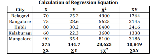
Regression equation of Y on X: Y = a + bX
The two normal equations are:
∑Y = Na + b∑X
∑XY = a∑X + b∑X2
Substituting the values in above normal equations, we get
141.7 = 5a + 375b ..... (i)
10849= 375a + 28625b ..... (ii)
Let us solve these equations (i) and (ii) by simultaneous equation method
Multiply equation (i) by 75 we get 10627.5 = 375a + 28125b
Now rewriting these equations:
10627.5 = 375a + 28125b
10849 = 375a + 28625b
(-) (-) (-) .
-221.5 = -500b
Therefore now we have -221.5 = -500b, this can rewritten as 500b = 221.5
Now, b = 221.5/500 = 0.443
Substituting the value of b in equation (i), we get
141.7 = 5a + (375 * 0.443)
141.7 = 5a + 166.125
5a = 141.7 - 166.125
5a = -24.425
a = -24.425/5
a = -4.885
Thus we got the values of a = -4.885 and b = 0.443
Hence, the required regression equation of Y on X:
Y = a + bX => Y = -4.885 + 0.443X
Estimated sales of automobiles (Y) in city Belagavi for the year 2020, where number of
families (X) are 100(in lakhs):
Y = -4.885 + 0.443X
Y = -4.885 + (0.443 * 100)
Y = -4.885 + 44.3
Y = 39.415 (‘000)
Means sales of automobiles would be 39,415 when number of families are 100,00,000
Example 4
Given below are five observation collected in simple regression. Calculate the intercept, slope and write down the estimated regression equation
X | Y |
2 | 7 |
4 | 5 |
6 | 4 |
8 | 2 |
10 | 1 |
Solution
X | Y | X2 | y2 | xy |
2 | 7 | 4 | 49 | 14 |
4 | 5 | 16 | 25 | 20 |
6 | 4 | 36 | 16 | 24 |
8 | 2 | 64 | 4 | 16 |
10 | 1 | 100 | 1 | 10 |
30 | 19 | 220 | 95 | 84 |
To find a and b, use the following equation
Find a:
((19 × 220) – ((30 × 84)) / 5 (220) – 900)
1660/ 200
=8.3
Find b:
(5(84) – (30 × 19)) / (5 (220) – 900)
-150 / 200
= -0.75
y’ = a + bx
y’ = 8.3 + (-0.75)x
Key takeaways - The quantity “b” in the regression equation is called as the regression coefficient or slope coefficient.
Sources


