3.1 Probability definition objective and subjective approachs addition and multiplication theorem of probability permutation and combination conditional probability Bays theorem

UNIT-III

Probability

3.1 Probability - definition, objective and subjective approachs, addition and multiplication theorem of probability, permutation and combination, conditional probability, Bay's theorem

Probability theory was originated from gambling theory. Probability is the measure of the likelihood that an event will occur in a Random Experiment. Probability is quantified as a number between 0 and 1, where, loosely speaking, 0 indicates impossibility and 1 indicates certainty. The higher the probability of an event, the more likely it is that the event will occur.

Example:

A simple example is the tossing of a fair (unbiased) coin. Since the coin is fair, the two outcomes (“heads” and “tails”) are both equally probable; the probability of “heads” equals the probability of “tails”; and since no other outcomes are possible, the probability of either “heads” or “tails” is 1/2 (which could also be written as 0.5 or 50%).

The probability formula is defined as the possibility of an event to happen is equal to the ratio of the number of favourable outcomes and the total number of outcomes.

Probability of event to happen P(E) = Number of favourable outcomes/Total Number of outcomes

Objective and subjective approach

Objective probability refers to estimating the likelihood that something will happen by using observations that we have recorded. A subjective probability or subjective estimate, on the other hand, is a guess which we base on personal experience. In other words, subjective measures use personal estimates, while objective measures use observations of what happened in the past.

Objective probability is the probability an event will occur based on an analysis in which each measure is based on a recorded observation or a long history of collected data.

Subjective probability - Subjective probability is a type of probability derived from an individual's personal judgment or own experience about whether a specific outcome is likely to occur. It contains no formal calculations and only reflects the subject's opinions and past experience.

Addition and multiplication theorem of probability,

Addition rule

𝑃(𝐴 ∪ 𝐵) = 𝑃(𝐴) + 𝑃(𝐵) − 𝑃(𝐴 ∩ 𝐵)

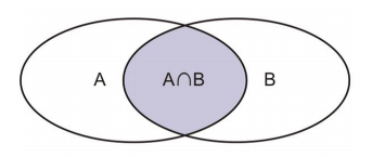
The probability of event A or event B can be found by adding the probability of the separate events A and B and subtracting any intersection of the two events.

More intuitively, if we were to take the area of the Venn Diagram below, we would add the areas of figures A and B, and subtract out one overlap’s worth of area, which represents the intersection of A and B.

Multiplication rule:

P(A and B) = 𝑃(𝐴) ∗ 𝑃(𝐵|𝐴)

The probability of events A and B occurring can be found by taking the probability of event A occurring and multiplying it by the probability of event B happening given that event A already happened.

If events A and B are independent, simply multiply (𝐴) by 𝑃(𝐵).

Example 1

If P(A) = 1/5 P(B/A) = 1/3. Then what is P(AnB)

Solution

P(A and B) = 𝑃(𝐴) ∗ 𝑃(𝐵|𝐴)

= 1/5*1/3 = 1/15

Example 2

From a pack of 52 cards, two cards are drawn at random one after the other with replacement. What is the probability that both cards are kings?

Solution

The probability of drawing a king P (A) =

The probability of drawing again the king after replacement P (B) =

Since the two events are independent, the probability of drawing two kings is:

Example 3

A bag contains 4 red balls, 3 white balls and 5 black balls. Two balls are drawn one after the other with replacement. Find the probability that first is red and the second is black.

Solution

Probability of red ball in the first draw =

The probability of a black ball in the second draw =

Since the events are independent, the probability that first is red and the second are black will be:

Example 4

A bag contains 5 white and 3 red balls and four balls are successively drawn and are not replaced. What is the chance that (i) white and red balls appear alternatively and (ii) red and white balls appear alternatively?

Solution

(i) The probability of drawing a white ball = 5/8

The probability of drawing a red ball = 3/7

The probability of drawing a white ball = 4/6 and the probability of drawing a red ball = 2/5

Since the events are dependent, therefore the required probability is:

(ii) The probability of drawing a red ball = 3/8 and the probability of drawing a white ball = 5/7

The probability of drawing a red ball = 2/6 and the probability of drawing a white ball = 4/5

Since the events are dependent, therefore the required probability is:

Permutation and combination:

Permutation and combination are very important concept in mathematics. It represents a group of objects by selecting them in a set and forming subsets. It defines the various ways to arrange a certain group of data. Permutation refers to when we select the data or objects from a certain group, whereas the order in which they are represented is called combination.

Permutation-

In mathematics, permutation relates to the act of arranging all the members of a set into some sequence or order. Permutations occur, in more or less prominent ways, in almost every area of mathematics. They often arise when different orderings on certain finite sets are considered.

Combination-

The combination is a way of selecting items from a collection, such that (unlike permutations) the order of selection does not matter. Combination refers to the combination of n things taken k at a time without repetition.

Example 1

Find the number of permutations and combinations if n = 12 and r = 2.

Solution:

Given,

n = 12

r = 2

Using the formula given above:

Permutation:

Combination:

Conditional probability

Let A and B be two events associated with a random experiment. Then, the probability of occurrence of A under the condition that B has already occurred and P(B) ≠ 0, is called the conditional probability and it is denoted by P(A/B).
Thus, P(A/B) = Probability of occurrence of A, given that B has already happened.
What are Addition and Multiplication Theorems on Probability 4
Similarly, P(B/A) = Probability of occurrence of B, given that A has already happened.

Sometimes, P(A/B) is also used to denote the probability of occurrence of A when B occurs. Similarly, P(B/A) is used to denote the probability of occurrence of B when A occurs.

Example 1

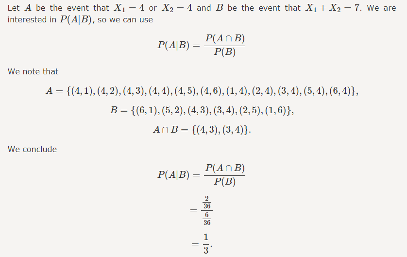
I roll a fair die twice and obtain two numbers X1= result of the first roll and X2= result of the second roll. Given that I know X1+X2=7, what is the probability that X1=4 or X2=4?

Solution

Example 2

I roll a fair die. Let A be the event that the outcome is an odd number, i.e., A={1,3,5}. Also let B be the event that the outcome is less than or equal to 3, i.e., B={1,2,3}. What is the probability of A, P(A)? What is the probability of A given B, P(A|B)?

Solution

This is a finite sample space, so

P(A)=|A|/|S|=|{1,3,5}|/6=12.

Now, let's find the conditional probability of A given that B occurred. If we know B has occurred, the outcome must be among {1,2,3}. For A to also happen the outcome must be in A∩B={1,3}. Since all die rolls are equally likely, we argue that P(A|B) must be equal to

P(A|B)=|A∩B|/|B|=23.

Bay's theorem:

In statistics and probability theory, the Bayes’ theorem (also known as the Bayes’ rule) is a mathematical formula used to determine the conditional probability of events. Essentially, the Bayes’ theorem describes the probability of an event based on prior knowledge of the conditions that might be relevant to the event.

The theorem is named after English statistician, Thomas Bayes, who discovered the formula in 1763. It is considered the foundation of the special statistical inference approach called the Bayes’ inference.

Formula for Bayes’ Theorem

Where,

a) P(A|B) – the probability of event A occurring, given event B has occurred.

b) P(B|A) – the probability of event B occurring, given event A has occurred.

c) P(A) – the probability of event A.

d) P(B) – the probability of event B.

Note that events A and B are independent events (i.e., the probability of the outcome of event A does not depend on the probability of the outcome of event B).

A special case of the Bayes’ theorem is when event A is a binary variable. In such a case, the theorem is expressed in the following way:

Where:

P(B|A–) – the probability of event B occurring given that event A– has occurred

P(B|A+) – the probability of event B occurring given that event A+ has occurred

In the special case above, events A– and A+ are mutually exclusive outcomes of event A.

Example 1

A bag I contain 4 white and 6 black balls while another Bag II contains 4 white and 3 black balls. One ball is drawn at random from one of the bags, and it is found to be black. Find the probability that it was drawn from Bag I.

Solution

Let E1 be the event of choosing the bag I, E2 the event of choosing the bag II, and A be the event of drawing a black ball.

Then,P(E1) = P(E2) = 1/2

Also,P(A|E1) = P(drawing a black ball from Bag I) = 6/10 = 3/5

P(A|E2) = P(drawing a black ball from Bag II) = 3/7

By using Bayes’ theorem, the probability of drawing a black ball from bag I out of two bags,

P(E1|A) = P(E1)P(A|E1)P(E1)P(A│E1)+P(E2)P(A|E2)

=(1/2 × 3/5)/(1/2 × 3/5 + 1/2 × 3/7) = 7/12

Example 2

A man is known to speak truth 2 out of 3 times. He throws a die and reports that the number obtained is a four. Find the probability that the number obtained is actually a four.

Solution

Let A be the event that the man reports that number four is obtained.

Let E1 be the event that four is obtained and E2 be its complementary event.

Then, P(E1) = Probability that four occurs = 1/6

P(E2) = Probability that four does not occurs = 1 – P(E1) = 1 −1/6 = 5/6

Also, P(A|E1) = Probability that man reports four and it is actually a four = 2/3

P(A|E2) = Probability that man reports four and it is not a four = 1/3

By using Bayes’ theorem, probability that number obtained is actually a four,

P(E1|A) =P(E1)P(A|E1)P(E1)P(A│E1) + P(E2)P(A|E2) = (1/6 × 2/3)/(1/6 × 2/3 + 5/6 × 1/3) = 2/7

Key takeaways –

The study of permutations and combinations is concerned with determining the number of different ways of arranging and selecting objects out of a given number of objects, without actually listing them.

3.2 Probability Distribution: Binomial, Poisson and Normal Distribution-Properties and applications.

Binominal distribution

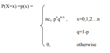
Binomial distribution was discovered by James Bernoulli (1654-1705). Let a random experiment be performed repeatedly and the occurrence of an event in a trial be called as success and its non-occurrence is failure. Consider a set of n independent trails (n being finite), in which the probability p of success in any trail is constant for each trial. Then q=1-p is the probability of failure in any trail.

The probability of x success and consequently n-x failures in n independent trails.

But x successes in n trails can occur in ncx ways. Probability for each of these ways is

pxqn-x

P(sss…ff…fsf…f)=p(s)p(s)….p(f)p(f)….

= p,p…q,q…

= (p,p…p)(q,q…q)

(x times) (n-x times)

Hence the probability of x success in n trials is given by

ncx pxqn-x

Definition:

A random variable x is said to follow binomial distribution if it assumes nonnegative values and its probability mass function is given by

The two independent constants n and p in the distribution are known as the parameters of the distribution.

Condition for Binomial distribution

We get the binomial distribution under the following experimentation conditions

The number of trial n is finite.

The trials are independent of each other.

The probability of success p is constant for each trial.

Each trial must result in a success or failure.

The events are discrete events.

Properties

If p and q are equal, the given binomial distribution will be symmetrical. If p and q are not equal, the distribution will be skewed distribution.

Mean = E(x) = np .

Variance =V(x) = npq (mean>variance) .

Application

Quality control measures and sampling process in industries to classify items as defectives or non-defective.

Medical applications such as success or failure, cure or no-cure.

Example 1

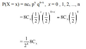
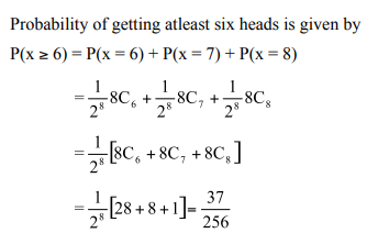
Eight coins are tossed simultaneously. Find the probability of getting atleast six heads.

Solution

Here number of trials, n = 8, p denotes the probability of getting a head.

∴ P = ½ and Q = 1/2

If the random variable X denotes the number of heads, then the probability of a success in n trials is given by

Example 2

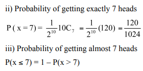
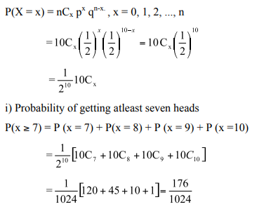
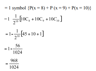
Ten coins are tossed simultaneously. Find the probability of getting (i) atleast seven heads (ii) exactly seven heads (iii) atmost seven heads

Solution

p = Probability of getting a head = ½ 2

q = Probability of not getting a head =1/2

The probability of getting x heads throwing 10 coins simultaneously is given by

Poission distribution:

The Poisson distribution, named after Simeon Denis Poisson (1781-1840). Poisson distribution is a discrete distribution. It describes random events that occurs rarely over a unit of time or space.

It differs from the binomial distribution in the sense that we count the number of success and number of failures, while in Poisson distribution, the average number of success in given unit of time or space

Definition:

The probability that exactly x events will occur in a given time is as follows

called as probability mass function of Poisson distribution.

Condition for Poisson distribution

Poisson distribution is the limiting case of binomial distribution under the following assumptions.

The number of trials n should be indefinitely large ie., n->∞

The probability of success p for each trial is indefinitely small.

np= λ, should be finite where λ is constant.

Properties:

Poisson distribution is defined by single parameter λ.

Mean = λ

Variance = λ. Mean and Variance are equal.

Application:

It is used in quality control statistics to count the number of defects of an item.

In biology, to count the number of bacteria.

In determining the number of deaths in a district in a given period, by rare disease.

The number of errors per page in typed material.

The number of plants infected with a particular disease in a plot of field.

Number of weeds in particular species in different plots of a field.

Example 1

Suppose on an average 1 house in 1000 in a certain district has a fire during a year. If there are 2000 houses in that district, what is the probability that exactly 5 houses will have a fire during the year? [given that e-2 = 0.13534]

Solution

Example 2

If 2% of electric bulbs manufactured by a certain company are defective. Find the probability that in a sample of 200 bulbs i) less than 2 bulbs ii) more than 3 bulbs are defective.[e-4 = 0.0183]

Solution

Normal distribution

Continuous Probability distribution is normal distribution. It is also known as error law or Normal law or Laplacian law or Gaussian distribution. Many of the sampling distribution like student-t, f distribution and χ2 distribution.

Definition

A continuous random variable x is said to be a normal distribution with parameters µ and σ 2 , if the density function is given by the probability law

Note:

The mean m and standard deviation s are called the parameters of Normal distribution.

The normal distribution is expressed by X ~ N(m, s2)

Condition

i) Normal distribution is a limiting form of the binomial distribution under the following conditions.

a) n, the number of trials is indefinitely large ie., nà¥ and

b) Neither p nor q is very small.

ii) Normal distribution can also be obtained as a limiting form of Poisson distribution with parameter mà¥

iii) Constants of normal distribution are mean = m, variation =s2 , Standard deviation = s

Normal probability curve

The curve representing the normal distribution is called the normal probability curve. The curve is symmetrical about the mean (m), bell-shaped and the two tails on the right and left sides of the mean extends to the infinity. The shape of the curve is shown in the following figure.

Properties

The normal curve is symmetrical about the mean μ;

The mean is at the middle and divides the area into halves;

The total area under the curve is equal to 1;

It is completely determined by its mean and standard deviation σ (or variance σ2).

The standard normal distribution:

A normal distribution is determined by ma and s. this creates a family of distributions depending on whatever the values of m and s are. The standard normal distribution has m = 0 and s = 1.

Formula

Example 1

In a normal distribution whose mean is 12 and standard deviation is 2. Find the probability for the interval from x = 9.6 to x = 13.8

Solution

Example 2

For a normal distribution whose mean is 2 and standard deviation 3. Find the value of the variate such that the probability of the variate from the mean to the value is 0.4115

Solution