UNIT –IV
Time Series Analysis
Introduction
A time series is set of data collected at successive point in a time or over successive period of time. A time series is a collection of observations made sequentially through time. The interval between observations can be any time interval (hours within days, weeks, months, years, etc.).
Some examples of time series are:
a) An analysis of a single sequence of data is called univariate time-series analysis.
b) An analysis of several sets of data for the same sequence of time periods is called multivariate time-series analysis or, more simply, multiple time-series analysis.
Utilities of time series:
1. It helps in understanding past behaviour and is useful for prediction of future.
2. It facilitates comparison.
3. The various components of time series are useful to study the effective change under each component.
4. The reasons for variation can be studied by comparing actual with expected results.
COMPONENT OF TIME SERIES
Fluctuation in a time series is mainly due to four basic components.
1 Secular trend or trend (T)
2 Seasonal variation (S)
3 Cyclical variation or cyclic fluctuation (C)
4 Irregular or random moments (I)
Secular trend or trend (T):
Seasonal Variation:
Cyclic Components:
Irregular Variation:
How the component relates to the original series?
A model that expresses the time series variable Y in terms of the components T (trend), C (cycle), S (seasonal) and I (irregular).
Measurement of trend:
1. Graphical method –
Under this method the values of a time series are plotted on a graph paper by taking time variable on the X-axis and the values variable on the Y-axis. After this, a smooth curve is drawn with free hand through the plotted points. The trend line drawn above can be extended to forecast the values. The following points must be kept in mind in drawing the freehand smooth curve.
(i) The curve should be smooth
(ii) The number of points above the line or curve should be approximately equal to the points below it
(iii) The sum of the squares of the vertical deviation of the points above the smoothed line is equal to the sum of the squares of the vertical deviation of the points below the line.
Merits
a) It is simple method of estimating trend.
b) It requires no mathematical calculations.
c) This method can be used even if trend is not linear.
Demerits
a) It is a subjective method.
b) The values of trend obtained by different statisticians would be different and hence not reliable.
Method of least Squares and curve fitting | ||||||||||||||||||||
|
| |||||||||||||||||||
It is a mathematical method and with it gives a fitted trend line for the set of data in such a manner that the following two conditions are satisfied.
This method gives the line which is the line of best fit. This method is applicable to give results either to fit a straight-line trend or a parabolic trend. The method of least squares as studied in time series analysis is used to find the trend line of best fit to a time series data. Secular Trend Line The secular trend line (Y) is defined by the following equation: Y = a + b X Where, Y = predicted value of the dependent variable a = Y-axis intercept i.e. the height of the line above origin (when X = 0, Y = a) b = slope of the line (the rate of change in Y for a given change in X) When b is positive the slope is upwards, when b is negative, the slope is downwards X = independent variable (in this case it is time) To estimate the constants a and b, the following two equations have to be solved simultaneously: ΣY = na + b ΣX ΣXY = aΣX + bΣX2
To simplify the calculations, if the midpoint of the time series is taken as origin, then the negative values in the first half of the series balance out the positive values in the second half so that ΣX = 0. In this case, the above two normal equations will be as follows: ΣY = na ΣXY = bΣX2
| ||||||||||||||||||||
Example: Below are given the figures of production (in thousand quintals) of a sugar factory: | ||||||||||||||||||||
| ||||||||||||||||||||
(a) Fit a straight-line trend to these figures. (b) Plot these figures on a graph and show the trend line. (c) Estimate the production in 2001.
| ||||||||||||||||||||
(d) Using normal equations and the sugar production data we can compute constants a and b as shown in Table 7.6:
Table : Calculations for Least Squares Equation
| ||||||||||||||||||||
| ||||||||||||||||||||
| ||||||||||||||||||||
| ||||||||||||||||||||
Therefore, linear trend component for the production of sugar is: | ||||||||||||||||||||
| ||||||||||||||||||||
| ||||||||||||||||||||
| ||||||||||||||||||||
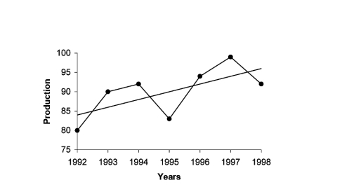
Fig.7.4: Linear Trend for Production of Sugar | ||||||||||||||||||||
| ||||||||||||||||||||
Plotting points on the graph paper, we get an actual graph representing production of sugar over the past 7 years. Join the point a = 82 and b = 2 (corresponds to 1993) on the graph we get a trend line as shown in Fig. 7.4. | ||||||||||||||||||||
| ||||||||||||||||||||
The production of sugar for year 2001 will be
| ||||||||||||||||||||
Parabolic Trend Model:
| ||||||||||||||||||||
The curvilinear relationship for estimating the value of a dependent variable y from an independent variable x might take the form | ||||||||||||||||||||
| ||||||||||||||||||||
This trend line is called the parabola.
For a non-linear equation
| ||||||||||||||||||||
| ||||||||||||||||||||
| ||||||||||||||||||||
| ||||||||||||||||||||
Example: The prices of a commodity during 1999-2004 are given below. Fit a parabola to these data. Estimate the price of the commodity for the year 2005.
Also plot the actual and trend values on a graph.
| ||||||||||||||||||||
Exponential trend model | ||||||||||||||||||||
Logarithm y = aebx. The equation is
Key Takeaways:
Y = a + b X.
| ||||||||||||||||||||
A moving average is a technique to get an overall idea of the trends in a data set; it is an average of any subset of numbers. The moving average is extremely useful for forecasting long-term trends. You can calculate it for any period of time. For example, if you have sales data for a twenty-year period, you can calculate a five-year moving average, a four-year moving average, a three-year moving average and so on. Stock market analysts will often use a 50 or 200 day moving average to help them see trends in the stock market and (hopefully) forecast where the stocks are headed.
An average represents the “middling” value of a set of numbers. The moving average is exactly the same, but the average is calculated several times for several subsets of data. For example, if you want a two-year moving average for a data set from 2000, 2001, 2002 and 2003 you would find averages for the subsets 2000/2001, 2001/2002 and 2002/2003. Moving averages are usually plotted and are best visualized.

Solution:
Computation of three- yearly moving averages.

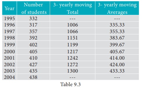
Example 9.5
Calculate four-yearly moving averages of number of students studying in a higher secondary school in a particular city from the following data.
Solution:
Computation of four- yearly moving averages.

Method of Least Square:
The line of best fit is a line from which the sum of the deviations of various points is zero. This is the best method for obtaining the trend values. It gives a convenient basis for calculating the line of best fit for the time series. It is a mathematical method for measuring trend. Further the sum of the squares of these deviations would be least when compared with other fitting methods. So, this method is known as the Method of Least Squares and satisfies the following conditions:
(i) The sum of the deviations of the actual values of Y and Ŷ (estimated value of Y) is Zero. that is Σ(Y–Ŷ) = 0.
(ii) The sum of squares of the deviations of the actual values of Y and Ŷ (estimated value of Y) is least. that is Σ(Y–Ŷ)2 is least ;
Procedure:
(i) The straight line trend is represented by the equation Y = a + bX …(1)
where Y is the actual value, X is time, a, b are constants
(ii) The constants ‘a’ and ‘b’ are estimated by solving the following two normal
Equations ΣY = n a + b ΣX ...(2)
ΣXY = a ΣX + b ΣX2 ...(3)
Where ‘n’ = number of years given in the data.
(iii) By taking the mid-point of the time as the origin, we get ΣX = 0
(iv) When ΣX = 0 , the two normal equations reduces to
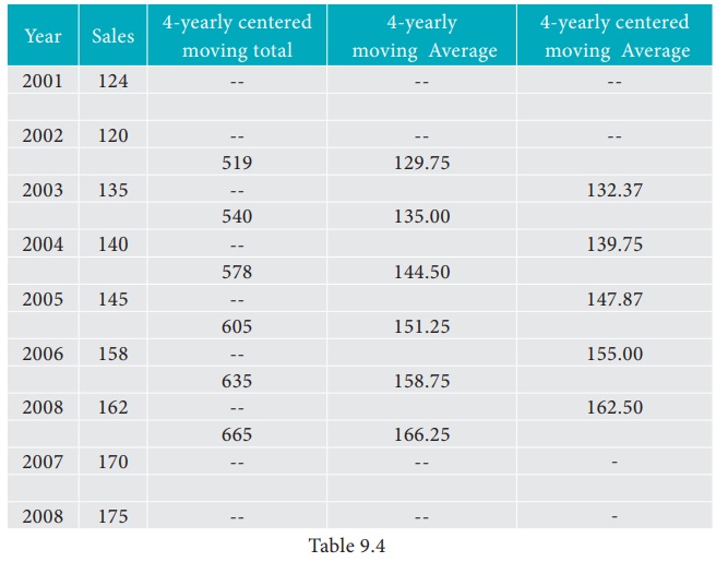
The constant ‘a’ gives the mean of Y and ‘b’ gives the rate of change (slope).
(v) By substituting the values of ‘a’ and ‘b’ in the trend equation (1), we get the Line of Best Fit.
Fit a straight-line trend by the method of least squares and tabulate the trend values.
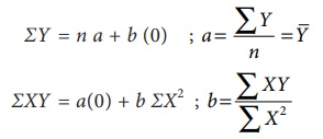
Solution:
Computation of trend values by the method of least squares (ODD Years).

Therefore, the required equation of the straight-line trend is given by
Y = a+bX;
Y = 45.143 + 1.036 (x-2003)
The trend values can be obtained by
When X = 2000, Yt = 45.143 + 1.036(2000–2003) = 42.035
When X = 2001, Yt = 45.143 + 1.036(2001–2003) = 43.071,
similarly, other values can be obtained.
2. Given below are the data relating to the sales of a product in a district.
Fit a straight-line trend by the method of least squares and tabulate the trend values.
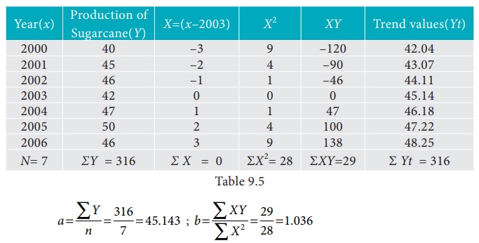
Solution:
Computation of trend values by the method of least squares.
In case of EVEN number of years, let us consider
 similarly other values can be obtained.
Key Takeaways:
Seasonal variations- estimation of seasonal variations
Seasonal variations occur in the time series due to the rhythmic forces which occurs in a regular and a periodic manner with in a period of less than one year. Seasonal variations occur during a period of one year and have the same pattern year after year. Here the period of time may be monthly, weekly or hourly. But if the figure is given in yearly terms then seasonal fluctuations does not exist. There occur seasonal fluctuations in a time series due to two factors.
1) Due to natural forces.
2) Man made convention.
The most important factor causing seasonal variations is the climate changes in the climate and weather conditions such as rain fall, humidity, heat etc. act on different products and industries differently.
For example, during winter there is greater demand for woolen clothes, hot drinks etc. Where as in summer cotton clothes, cold drinks have a greater sale and in rainy season umbrellas and rain coats have greater demand.
Though nature is primarily responsible for seasonal variation in time series, customs, traditions and habits also have their impact. For example, on occasions like dipawali, dusserah, Christmas etc. there is a big demand for sweets and clothes etc., there is a large demand for books and stationary in the first few months of the opening of schools and colleges.
Methods of simple averages
This is the simplest of all the methods of measuring seasonality. This method is based on the additive modal of the time series. That is the observed values of the series is expressed by Yt = RtCt St Tt and in this method we assume that the trend component and the cyclical component are absent.
The method consists of the following steps-


Merits and Demerits:
Method of simple average is easy and simple to execute.
This method is based on the basic assumption that the data do not contain any trend and cyclic components. Since most of the economic and business time series have trends and as such this method though simple is not of much practical utility.
Example
Assuming that the trend is absent, determine if there is any seasonality in the data given below.

Ratio to trend method:
This method is an improvement over the simple averages method and this method assumes a multiplicative model i.e
The measurement of seasonal indices by this method consists of the following steps.
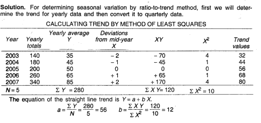
1. Obtain the trend values by the least square method by fitting a mathematical curve, either a straight line or second-degree polynomial.
2. Express the original data as the percentage of the trend values. Assuming the multiplicative model these percentages will contain the seasonal, cyclical and irregular components.
3. The cyclical and irregular components are eliminated by averaging the percentages for different months (quarters) if the data are In monthly (quarterly), thus leaving us with indices of seasonal variations.
4. Finally these indices obtained in step(3) are adjusted to a total of 1200 for monthly and 400 for quarterly data by multiplying them through out by a constant K which is given by

Example
Determine seasonal variation through ratio to trend method

Solution

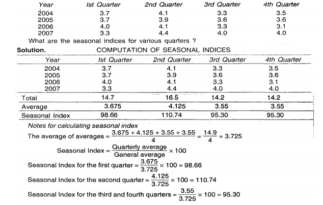
Ratio to moving average method
The ratio to moving average method is also known as percentage of moving average method and is the most widely used method of measuring seasonal variations. The steps necessary for determining seasonal variations by this method are
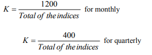
1. Calculate the centered 12-monthly moving average (or 4-quarterly moving average) of the given data. These moving averages values will eliminate S and I leaving us T and C components.
2. Express the original data as percentages of the centered moving average values.
3. The seasonal indices are now obtained by eliminating the irregular or random components by averaging these percentages using A.M or median.
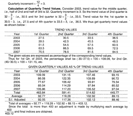
4. The sum of these indices will not in general be equal to 1200 (for monthly) or 400 (for quarterly). Finally the adjustment is done to make the sum of the indices to a total of 1200 for monthly and 400 for quarterly data by multiplying them through out by a constant K which is given by
Example-
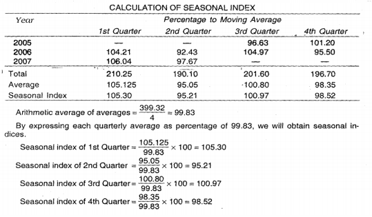
Calculate seasonal indices by the ratio to moving average method, from the following data

Key takeaways - The ratio-to-moving-average method, the trend values are obtained by the method of moving averages, in the ratio-to-trend method, the corresponding trend is obtained by the method of least sequares.
The value of money does not remain same over the time. A rise in the price levels means a fall in the value of money and a fall in the price level means a rise in the value of money. Thus index number is a statistical device that measures the relative change in the level of price from one time period to another.
Definition:
“Index numbers are quantitative measures of growth of prices, production, inventory and other quantities of economic interest” ………Ronold
An index number measures how much a variable changes over the time. Index number is calculated by finding the ratio of current value to a base value.
Uses of index number
(a) Index numbers are specialized averages.
(b) Index numbers measures the change in one variable or a group of variables.
(c) Index numbers measures the effect of changes over a period of time.
(d) Index numbers are meant to study the changes in the effects of such factors which cannot be measured directly.
Construction of index number:
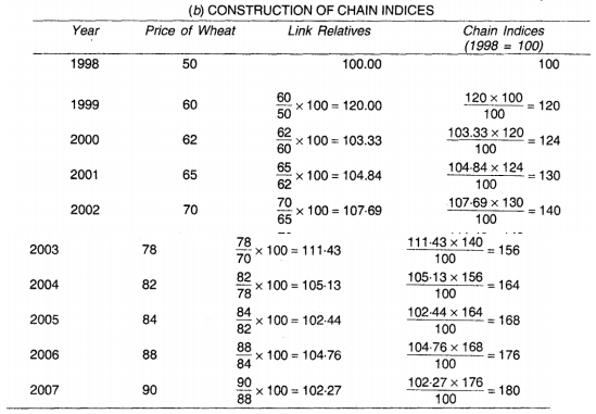
The chain index numbers - In fixed base method the base remain constant through out i.e. the relatives for all the years are based on the price of that single year. On the other hand in chain base method, the relatives for each year is found from the prices of the immediately preceding year. Thus, the base changes from year to year. Such index numbers are useful in comparing current year figures with the preceding year figures. The relatives which we found by this method are called link relatives.
Thus, link relative for current year = current years’ figure/previous year figure *100
And by using these link relatives we can find the chain indices for each year by using the below formula
Chain index for current year = Link relative of current year * Chain index of previous year/ 100
Note: The fixed base index number computed from the original data and chain index number computed from link relatives give the same value of the index provided that there is only one commodity, whose indices are being constructed.
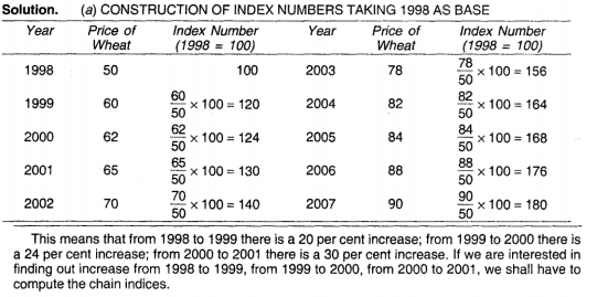
Example 1
From the following data of wholesale prices of wheat for ten years construct index number taking a) 1998 as base and b) by chain base method

Example 2
From the following data calculate the index numbers using the Chain Index Numbers method.
Year 2011 2012 2013 2014 2015 2016 2017 2018
Prices 120 124 130 144 150 160 164 170
Solution
Construction of Chain Index Numbers
Year | Price | Link Relatives | Chain indices |
2011 | 120 | 100 | 100 |
2012 | 124 | 120/124 x 100 = 103.33 | 103.33 ×100/100 = 103.33 |
2013 | 130 | 124/130 x 100 = 104.83 | 104.83 ×103.33/100 = 108.32 |
2014 | 144 | 130/144 x 100 = 110.76 | 110.76×108.32 /100= 119.98 |
2015 | 150 | 144/150 x 100 = 104.16 | 104.16 ×119.98/100 = 124.97 |
2016 | 160 | 150/160 x 100 = 106.66 | 106.66×124.97/100 = 133.29 |
2017 | 164 | 160/164 x 100 = 102.5 | 102.5 ×133.29/100 = 136.62 |
2018 | 170 | 164/170 x 100 = 103.65 | 103.65 ×136.62/100 = 141.61 |
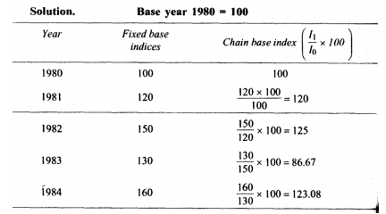
Example 3
Compute the chain base index numbers
Solution

Fixed base method – under this method index number is calculated with a fixed base year. By this method the index number of a given year is not influenced by the variation of prices of any other year.
Price relatrive of current year = price of current year/ price of base year*100
Example 1
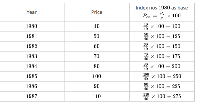
Find index numbers for the following data taking 1980 as the base year.
Year | 1980 | 1981 | 1982 | 1983 | 1984 | 1985 | 1986 | 1987 |
Price | 40 | 50 | 60 | 70 | 80 | 100 | 90 | 110 |
Solution

Construction of price index numbers:
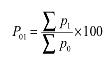
Where, P01 = Index number
P 1= Total of the current year’s prices of all commodities
P 0= Total of the base year’s prices of all commodities
Example 1
Commodity | Price in base year 2005 | Price in current year 2010 |
A | 10 | 20 |
B | 15 | 25 |
C | 40 | 60 |
D | 25 | 40 |
Solution
Commodity | Price in base year 2005 | Price in current year 2010 |
A | 10 | 20 |
B | 15 | 25 |
C | 40 | 60 |
D | 25 | 40 |
|
|
|
Index number ( P01 ) = 
P01 = (145/90)*100 = 161.11
It means the price in 2010 were 61% more than the price in 2005.
Example 2
Find the index number from the data given below
Commodities | Units | Price in 2007 | Price in 2008 |
Sugar | Quintal | 2200 | 3200 |
Milk | Quintal | 18 | 20 |
Oil | Liter | 68 | 71 |
Wheat | Quintal | 900 | 1000 |
Clothing | Meter | 50 | 60 |
|
|
|
|
Solution
Commodities | Units | Price in 2007 | Price in 2008 |
Sugar | Quintal | 2200 | 3200 |
Milk | Quintal | 18 | 20 |
Oil | Liter | 68 | 71 |
Wheat | Quintal | 900 | 1000 |
Clothing | Meter | 50 | 60 |
|
|
|
|
Index number ( P01 ) = 
P01 = (4351/3236)*100 = 134.45
It means the price in 2008 were 34% more than the price in 2007.
Example 3
Construct the price index for 2003, taking the year 2000 as base year
Commodities | Price in 2000 | Price in 2003 |
A | 60 | 80 |
B | 50 | 60 |
C | 70 | 100 |
D | 120 | 160 |
E | 100 | 150 |
|
|
|
Solution
Commodities | Price in 2000 - P 0 | Price in 2003 - P 1 |
A | 60 | 80 |
B | 50 | 60 |
C | 70 | 100 |
D | 120 | 160 |
E | 100 | 150 |
|
|
|
Index number (P01) = 
P01 = (550/400)*100 = 137.5
Therefore, there is an increase of 37.5% in the prices in 2003 as against 2000.
Example 4
Compute the price index for the years 2001, 2002, 2003, 2004 taking 2000 as base year
Year | 2000 | 2001 | 2002 | 2003 | 2004 |
Price | 120 | 144 | 168 | 204 | 216 |
Solution
Price index for different years
2000 | (120/120)*100 = 100 |
2001 | (144/120)*100 = 120 |
2002 | (168/120)*100 = 140 |
2003 | (204/120)*100 = 170 |
2004 | (216/120)*100 = 180 |
Example 5
Prepare simple aggregative price index
Commodities | Price in 1995 - P 0 | Price in 2003 - P 1 |
Wheat | 100 | 140 |
Rice | 200 | 250 |
Pulses | 250 | 350 |
Sugar | 14 | 20 |
Oil | 40 | 50 |
Solution
Commodities | Price in 1995 - P 0 | Price in 2003 - P 1 |
Wheat | 100 | 140 |
Rice | 200 | 250 |
Pulses | 250 | 350 |
Sugar | 14 | 20 |
Oil | 40 | 50 |
|
|
|
Simple aggregative index number = (810/604)*100 = 134.1
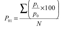
2. Simple average of relative method - in this method, index number is equal to the sum of price relatives divided by the number of items.

Where, N= number of items
Example 1
Commodity | Base year | Current year |
A | 10 | 20 |
B | 15 | 25 |
C | 40 | 60 |
D | 25 | 40 |
|
|
|
Solution
Commodity | Base year | Current year | Price relatives |
A | 10 | 20 | (20/10)*100 = 200 |
B | 15 | 25 | (25/15)*100 =166.7 |
C | 40 | 60 | (60/40)*100 =150 |
D | 25 | 40 | (40/25)*100 =160 |
N = 4 |
|
|
|

Index number = 676.7/4 = 169.2
Example 2
Construct the index number for the year 2010
Commodities | Price (2009) | Price(2010) |
P | 6 | 10 |
Q | 12 | 2 |
R | 4 | 6 |
S | 10 | 12 |
T | 8 | 12 |
|
|
|
Solution
Commodities | Price (2009) | Price(2010) | Price relative |
P | 6 | 10 | 166.67 |
Q | 12 | 2 | 16.67 |
R | 4 | 6 | 150 |
S | 10 | 12 | 120 |
T | 8 | 12 | 150 |
N = 5 |
|
| 603.34 |

Index number = 603.34/4 = 120.68.
Example 3
Using simple average of price relative method find price index for 2001, taking 1996 as base year for the following data
Commodity | Wheat | Rice | Sugar | Ghee | Tea |
Price in 1996 | 12 | 20 | 12 | 40 | 80 |
Price in 2001 | 16 | 25 | 16 | 60 | 96 |
Solution
Commodities | Price (2009) | Price(2010) | Price relative |
Wheat | 12 | 16 | (16/12)*100 = 133.33 |
Rice | 20 | 25 | (25/20)*100 = 125 |
Sugar | 12 | 16 | 133.33 |
Ghee | 40 | 60 | 150 |
Tea | 80 | 96 | 120 |
N = 5 |
|
| 661.66 |

 =661.66 = 132.33
5
Therefore Price Index for 2001, taking 1996 as base year, = 132.33
Example 4
Using simple average of price relative method find price index for 2010, taking 2009 as base year for the following data
Commodities | Price (2009) | Price(2010) |
A | 60 | 80 |
B | 50 | 60 |
C | 60 | 72 |
D | 50 | 75 |
E | 25 | 37 .5 |
F | 20 | 30 |
Solution
Commodities | Price (2009) | Price(2010) | Price relatives |
A | 60 | 80 | 133.33 |
B | 50 | 60 | 120 |
C | 60 | 72 | 120 |
D | 50 | 75 | 150 |
E | 25 | 37 .5 | 150 |
F | 20 | 30 | 150 |
N = 6 |
|
| 823.33 |

= 823.33/6 = 137.22
3. Weighted aggregative method – in this method, according to the relative importance, different weights are assigned to the items. Many formulas developed to estimate index numbers on the basis of weights.
Some of the formulas given below
(a) Laspeyre’s formula - In this method, the quantities of the base year are accepted as weight

(b) Paasche’s formula – in this method, the quantities of the current year are accepted as weight

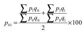
(c) Dorbish and Bowley’s formula – this method is the combination of Laspeyre’s formula and Paasche’s formula
(d) Fisher’s ideal formula – this method is the geometric mean of Laspeyre’s formula and Paasche’s formula

(e) Marshall – Edgeworth method - In this method also both the current year as well as base year prices and quantities are considered.

(f) Kelly’s method –

Where q refers to quantity of some period, not necessarily of the mean of the base year and current year.
Example 1
Commodity | Base year | Current year | ||
PO | QO | P1 | Q1 | |
A | 10 | 5 | 20 | 2 |
B | 15 | 4 | 25 | 8 |
C | 40 | 2 | 60 | 6 |
D | 25 | 3 | 40 | 4 |
Solution
Commodity | Base year | Current year |
|
|
|
| ||
PO | QO | P1 | Q1 | Poqo | P1qo | Poq1 | P1q1 | |
A | 10 | 5 | 20 | 2 | 50 | 100 | 20 | 40 |
B | 15 | 4 | 25 | 8 | 60 | 100 | 120 | 200 |
C | 40 | 2 | 60 | 6 | 80 | 120 | 240 | 360 |
D | 25 | 3 | 40 | 4 | 75 | 120 | 100 | 160 |
|
|
|
|
| 265 | 440 | 480 | 760 |
(a) Laspeyre’s formula

P 01 = (440/265)*100 = 166.04
(b) Paasche’s formula

P 01 = (760/480)*100 = 158.33
(c) Dorbish and Bowley’s formula

 P 01 = ((440/265) + (760/480)) *100 = 162
2
(d) Fisher’s ideal formula

 P 01 = √ ((440/265) + (760/480)) *100 = 162.1
Example 2
Commodity | Base year | Current year | ||
PO | QO | P1 | Q1 | |
A | 15 | 500 | 20 | 600 |
B | 18 | 590 | 23 | 640 |
C | 22 | 450 | 24 | 500 |
Solution
Commodity | Base year | Current year |
|
|
|
| ||
PO | QO | P1 | Q1 | Poqo | P1qo | Poq1 | P1q1 | |
A | 15 | 500 | 20 | 600 | 7500 | 10000 | 9000 | 12000 |
B | 18 | 590 | 23 | 640 | 10620 | 13570 | 11520 | 14720 |
C | 22 | 450 | 24 | 500 | 9900 | 10800 | 11000 | 12000 |
|
|
|
|
|
|
|
|
|
|
|
|
|
| 28020 | 34370 | 31520 | 38720 |
(a) Laspeyre’s formula
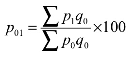
P 01 = (34370/28020)*100 = 122.66
(b) Paasche’s formula

P 01 = (38720/31520)*100 = 122.84
(c) Dorbish and Bowley’s formula

 P 01 = ((34370/28020) + (38720/31520)) *100 = 122.66
2
(d) Fisher’s ideal formula

 P 01 = √ = ((34370/28020) + (38720/31520)) *100 = 122.69
Example 3
Commodity | Base year | Current year | ||
PO | QO | P1 | Q1 | |
A | 2 | 8 | 4 | 6 |
B | 5 | 10 | 6 | 5 |
C | 4 | 14 | 5 | 10 |
D | 2 | 19 | 2 | 13 |
Solution
Commodity | Base year | Current year |
|
|
|
| ||
PO | QO | P1 | Q1 | Poqo | P1qo | Poq1 | P1q1 | |
A | 2 | 8 | 4 | 6 | 16 | 32 | 12 | 24 |
B | 5 | 10 | 6 | 5 | 50 | 60 | 25 | 30 |
C | 4 | 14 | 5 | 10 | 56 | 70 | 40 | 50 |
D | 2 | 19 | 2 | 13 | 38 | 38 | 26 | 26 |
|
|
|
|
| 160 | 200 | 103 | 130 |
|
|
|
|
|
|
|
|
|
(a) Laspeyre’s formula

P 01 = (200/160)*100 = 125
(b) Paasche’s formula
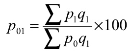
P 01 = (130/103)*100 = 126.21
(c) Dorbish and Bowley’s formula

 P 01 = ((200/160) + (130/103)) *100 = 125.6
2
(d) Fisher’s ideal formula
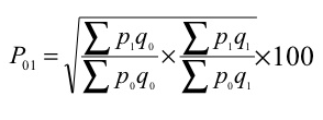
 P 01 = √ = ((200/160) + (130/103)) *100 = 125.61
(e) Marshall-Edgeworth method
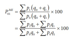
= (200+130)/(160+103) *100 = 125.48
Example 4
Calculate the price indices from the following data by applying (1) Laspeyre’s method (2) Paasche’s method and (3) Fisher ideal number by taking 2010 as the base year.
Commodity | 2010 | 2011 | ||
PO | QO | P1 | Q1 | |
A | 20 | 10 | 25 | 13 |
B | 50 | 8 | 60 | 7 |
C | 35 | 7 | 40 | 6 |
D | 25 | 5 | 35 | 4 |
Solution
Commodity | 2010 | 2011 |
|
|
|
| ||
PO | QO | P1 | Q1 | Poqo | P1qo | Poq1 | P1q1 | |
A | 20 | 10 | 25 | 13 | 200 | 250 | 260 | 325 |
B | 50 | 8 | 60 | 7 | 400 | 480 | 350 | 420 |
C | 35 | 7 | 40 | 6 | 245 | 280 | 210 | 240 |
D | 25 | 5 | 35 | 4 | 125 | 175 | 100 | 140 |
|
|
|
|
| 970 | 1185 | 920 | 1125 |
(a) Laspeyre’s formula

P 01 = (1185/970)*100 = 122.16
(b) Paasche’s formula

P 01 = (1125/920)*100 = 122.28
(c) Fisher’s ideal formula

 P 01 = √ = ((1185/970) + (1125/920)) *100 = 120.55
Example 5
Calculate the Dorbish and Bowley’s price index number for the following data taking 2014 as base year.
Item | 2010 | 2011 | ||
PO | QO | P1 | Q1 | |
Oil | 80 | 3 | 100 | 4 |
Pulses | 35 | 2 | 45 | 3 |
Sugar | 25 | 2 | 30 | 3 |
Rice | 50 | 30 | 54 | 35 |
Solution
Item | 2010 | 2011 |
|
|
|
| ||
PO | QO | P1 | Q1 | Poqo | P1qo | Poq1 | P1q1 | |
Oil | 80 | 3 | 100 | 4 | 240 | 300 | 320 | 400 |
Pulses | 35 | 2 | 45 | 3 | 70 | 90 | 105 | 135 |
Sugar | 25 | 2 | 30 | 3 | 50 | 60 | 75 | 90 |
Rice | 50 | 30 | 54 | 35 | 1500 | 1620 | 1750 | 1890 |
|
|
|
|
| 1860 | 2070 | 2250 | 2515 |
(d) Dorbish and Bowley’s formula

 P 01 = ((2070/1860) + (2515/2250)) *100 = 111.38
2
Example 6
Calculate a suitable price index from the following data
commodity | Quantity | price | |
|
| 2007 | 2010 |
X | 25 | 3 | 4 |
Y | 12 | 5 | 7 |
Z | 10 | 6 | 5 |
Solution
commodity | Q | P0 | P1 | P0Q | P1Q |
X | 25 | 3 | 4 | 75 | 100 |
Y | 12 | 5 | 7 | 60 | 84 |
Z | 10 | 6 | 5 | 60 | 50 |
|
|
|
| 195 | 234 |
Kelly price index

= 235/195*100 = 120
4. Weighted average of relative method – in this method different weights are used for the items according to their relative importance. If p = [p1/ p0] × 100 is the price relative index and w = p0q0 is attached to the commodity

Where,  means sum of weights for different commodities
 Sum of price relatives
Example 1
Commodity | Weight | Base price year | current price year |
A | 5 | 10 | 20 |
B | 4 | 15 | 25 |
C | 2 | 40 | 60 |
D | 3 | 25 | 40 |
Solution
Commodity | Weight | Base price year | current price year | price relatives | RW |
A | 5 | 10 | 20 | 20/10*100 = 200 | 1000 |
B | 4 | 15 | 25 | 25/15*100 =166.7 | 666.8 |
C | 2 | 40 | 60 | 60/40*100 = 150 | 300 |
D | 3 | 25 | 40 | 40/25*100 = 160 | 480 |
| 14 |
|
|
| 2446.8 |

P01 = 2446.8/14 = 174.8
Example 2
Compute price index by applying weighted average of relative method
Commodity | Quantity | Base price year | current price year |
Wheat | 20 | 3 | 4 |
Flour | 40 | 1.5 | 1.6 |
Milk | 10 | 1 | 1.5 |
Solution
Commodity | Quantity | Base price year | current price year | Weight | price relatives | RW |
Wheat | 20 | 3 | 4 | 60 | 133.3 | 8000 |
Flour | 40 | 1.5 | 1.6 | 60 | 106.7 | 6400 |
Milk | 10 | 1 | 1.5 | 10 | 150.0 | 1500 |
|
|
|
|
|
|
|
|
|
|
| 130 |
| 15900 |

P01 = 15900/130 = 122.30
Example 3
Calculate weighted average of relative method
Commodity | Base price year | current price year | Weight |
x | 3 | 4 | 7 |
y | 1.5 | 1.6 | 8 |
z | 1 | 1.5 | 9 |
Solution
Commodity | Base price year | current price year | Weight | price relatives | RW |
x | 3 | 4 | 7 | 133.3 | 933.33 |
y | 1.5 | 1.6 | 8 | 106.7 | 853.33 |
z | 1 | 1.5 | 9 | 150.0 | 1350 |
|
|
| 24 |
| 3136.66 |

P01 = 3136.66/24 = 130.67
Composite index number - A composite index number measures the variation in the value of a composite number defined as the aggregate of a set of elementary numbers (for example, the consumer price index measures the variation in the prices of 1,000 varieties of products in a single index number).
The composite index number is a weighted mean of the elementary index numbers in which the weighting represents the "mass" of the elementary numbers (in the case of price indices, this mass is expenditure).
A Laspeyres index is weighted according to mass in the base period.
A Paasche index is weighted according to mass in the current period.
Univariate index number - When index number is calculated from a single variable, it is called Univariate Index Number . The construction univariate index number is a simple idea.
Key takeaways –
Consumer price index
A consumer price index or cost of living index, is a measure which indicates the relative changes in the prices of a group of items, necessary for the living for a selected group of consumers. In a way, it tells us about what should be the increase in the wages of consumer so that they are able to maintain some standard of living in two time periods. For this purpose, the total expenditure of a household are categorized like food, clothing, rent, electricity, entertainment, education, medicines, miscellaneous etc.
Consumer Price Index number or Cost of living index number measures the effect of changes in the prices of the described basket of goods and services on the purchasing power of a particular class of people during current period as compared with some base period. Change in the cost of living of an individual between two periods means the change in his money income, which will be necessary for him to maintain the same standard of living in both periods. There the cost of living index numbers are intended to measure the average increase in the cost of maintaining the same standard in a given year as in the base year.
Computation of consumer price index number
For computing consumer Price Index no. or cost of living index no. we need to have prices and quantity consumed for different categories of items in base a year and current year.
Let
Poj = Price of jth commodity in 0 year (base year)
Pij = Price of jth commodity in I year (current year).
qoj = Quantity consumed for j th commodity in 0 year (base year)
Now, consumer Price Index no. is derived as the weighted average of the price relatives, the weight being the values of the quantities consumed in the base year. Price relative

Weight

Then,
Consumer Price Index

Example
Construct the cost of living index for the year 1982 (Base 1980 = 100).
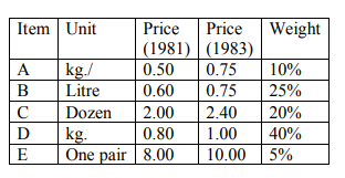
Solution
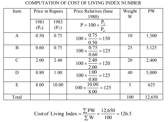
Key takeaways - Cost of Living Index Number or consumer’s price index number is a number which measures the average change in the retail price paid by a particular class of people at a particular place for a select of specified commodities and services, over two different time period.
Sources-
(a) I.B. N. Gupta: Business Math & Statistics.
(b) II. S. P. Singh: Statistics.
(c) III. Mukund Lal: Statistics.
(d) IV. K. N. Nayar: Statistics.
(e) V. C. B. Gupta: Statistics.
(f) VI. Shukla & Sahay: Statistical Analysis.
(g) VII. C. D. Gupta: Statistical Analysis.
(h) VIII. D. N. Elhana: Statistical Analysis.


