Unit 3
Production function
The term ‘production’ is extremely important and broader concept in economics. To satisfy the daily demand of a consumer production is essential part. Production is a process by which various inputs are combined and transformed into output of products and services, for which there's a demand in the market. In other words, Production is a process of mixing various material inputs and immaterial inputs in order to create something for consumption. The essences of production are the creation of utilities and therefore the transformation of inputs or resources into output. Inputs are the resources utilized in the production of goods and services the important resources or input in production are land, labour, capital, and entrepreneur. Production process creates economic well-being into the state. Thus, production is a process which creates utility and value in exchange.
The theory of production function is concern with the problem within the production process during a certain level of output. It analyses the relation between cost and output and help the firm to determine its profit. All firms that aim at maximising their profit must make their decision regarding production on the bases of the subsequent three decisions:
a. What quantity output to produce and supply in the market?
b. The way to produce the product, i.e. which technique of production or combination of production to used have to be decided?
c. How much quantity of input is demanded to supply the output of the product?
Thus, the above three decisions are interrelated and need to be taken by the firm during the production process.
In economics, a production function is that the functional relationship between physical output of a production process to physical inputs or factors of production. In other words, production function denotes an efficient combination of input and output. The factors which are utilized in the production of products and services are also called as agents of production. Production function of a business firm is decided by the state of technology. More specifically, production function shows the maximum volume of physical output available from a given set of inputs, or the minimum set of inputs necessary to supply any given level of output.
Definition: With the above statements we will define the production function as: “A production function refers to the functional relationship, under the given technology, between physical rates of input and output of firm, per unit of time”.
Mathematically, production function is express as: Q = f (N, L,K, E, T, etc.)
Production Function: Meaning, Definitions and Features
Production is the results of co-operation of 4 factors of production viz., land, labour, capital and organization.
This is evident from the fact that no single commodity is often produced without the help of anyone of these four factors of production.
Therefore, the producer combines all the four factors of production in a technical proportion. The aim of the producer is to maximise his profit. For this sake, he decides to maximise the production at minimum cost by means of the most effective combination of factors of production.
The producer secures the most effective combination by applying the principles of equi-marginal returns and substitution. Consistent with the principle of equi-marginal returns, any producer can have maximum production only when the marginal returns of all the factors of production are equal to one another. For example, when the marginal product of the land is equal to that of labour, capital and organisation, the production becomes maximum.
Meaning of Production Function:
In simple words, production function refers to the functional relationship between the amount of a good produced (output) and factors of production (inputs).
“The production function is only a technical relation which connects factor inputs and output.” Prof. Koutsoyiannis
Defined production function as “the relation between a firm’s physical production (output) and therefore the material factors of production (inputs)” Prof. Watson
In this way, production function reflects how much output we are able to expect if we've so much of labour then much of capital also as of labour etc. In other words, we will say that production function is an indicator of the physical relationship between the inputs and output of a firm.
The reason behind physical relationship is that money prices don't appear in it. However, here one thing that becomes most significant to quote is that like demand function a production function is for a definite period.
It shows the flow of inputs resulting into a flow of output during some time. The production function of a firm depends on the state of technology. With every development in technology the production function of the firm undergoes a change.
The new production function brought about by developing technology displays same inputs and more output or the same output with lesser inputs. Sometimes a new production function of the firm is also adverse because it takes more inputs to produce the same output.
Mathematically, such a basic relationship between inputs and outputs could also be expressed as:
Q = f( L, C, N )
Where Q = Quantity of output
L = Labour
C = Capital
N = Land.
Hence, the extent of output (Q), depends on the quantities of various inputs (L, C, N) available to the firm. Within the simplest case, where there are only two inputs, labour (L) and capital (C) and one output (Q), the production function becomes.
Q =f (L, C)
Definitions:
“The production function is a technical or engineering relation between input and output. As long because the natural laws of technology remain unchanged, the production function remains unchanged.” Prof. L.R. Klein
“Production function is the relationship between inputs of productive services per unit of time and outputs of product per unit of time.” Prof. George J. Stigler
“The relationship between inputs and outputs is summarized in what's called the production function. This is"> this is often a technological relation showing for a given state of technological knowledge what proportion can be produced with given amounts of inputs.” Prof. Richard J. Lipsey
Thus, from the above definitions, we will conclude that production function shows for a given state of technological knowledge, the relation between physical quantities of inputs and outputs achieved per period of time.
Features of Production Function:
Following are the features of production function:
1. Substitutability:
The factors of production or inputs are substitutes of 1 another which make it possible to vary the total output by changing the quantity of 1 or a few inputs, while the quantities of all other inputs are held constant. It's the substitutability of the factors of production that gives rise to the laws of variable proportions.
2. Complementarity:
The factors of production are complementary to one another, that is, the 2 or more inputs are to be used together as nothing will be produced if the quantity of either of the inputs utilized in the production process is zero.
The principle of returns to scale is another manifestation of complementarity of inputs because it reveals that the quantity of all inputs is to be increased simultaneously in order to achieve a higher scale of total output.
3. Specificity:
It reveals that the inputs are specific to the production of a specific product. Machines and equipment’s, specialized workers and raw materials are a few examples of the specificity of factors of production. The specificity might not be complete as factors is also used for production of other commodities too. This reveals that in the production process none of the factors are often ignored and in some cases ignorance to even slightest extent isn't possible if the factors are perfectly specific.
Production involves time; hence, the way the inputs are combined is determined to a large extent by the period of time under consideration. The greater the period of time, the greater the freedom the producer has to vary the quantities of varied inputs utilized in the production process.
In the production function, variation in total output by varying the quantities of all inputs is possible only in the long run whereas the variation in total output by varying the quantity of single input could also be possible even in the short run.
TYPES OF PRODUCTION FUNCTION
I. The production function is broadly categorised into two based on the time period i.e. a) Short run production function and b) long run production function.
A) Short run production function: The short run is defined as the period during which at least one among the input is fixed. Consistentwith the following short-run production function, labour is the only variable factor input while the rest of the inputs are considered fixed. In other words, the short run is a period in which the firm can adjust production by changing variable factors like materials and labour but cannot change fixed factors like land, capital, etc. Thus, in short-run some factors are fixed and some are variable.
B) Long run production function: The long run production function is defined because the period of time in which all factors of production are variable. In the long run there's no distinction between the fixed or variable factor as all factors in the long run are variable.
II. The production function can even be classified on the premise of factor proportion i.e.
a) Fixed proportion production function and
b) Variable proportion production function.
A. Fixed proportion production function: The fixed proportion production function, also referred to as a Leontief Production
Function which means the fixed factors of production function such as land, labour, raw materials are used to produce a fixed quantity of an output and these factors of production function cannot be substituted for the other factors. In other words, in such factors of production function fixed quantity of inputs is used to produce the fixed quantity of output. All factors of production are fixed and cannot be substituted for each other.
B. Variable proportion production function: The variableproportion production function supposes that the ratio in whichthe factors of production like labour and capital are utilized in a variable proportion. Also, the various combinations of factorscan be used to produce the given quantity, thus, one factor canbe substituted for the other factor. In the case of variableproportion production function, the technical Coefficient ofproduction function is variable, i.e. the important quantity ofoutput are often achieved through the combination of differentquantities of factors of production, like these factors are often varied by substituting one factors to the other/ factors in itsplace.
The term Iso-quant or Iso-product consists of two words, Iso = equal, quant = quantity or product = output.
Thus it means equal quantity or equal product. Various factors are needed to produce a good. These factors could also be substituted for each other.
A given quantity of output is also produced with different combinations of factors. Iso-quant curves also are referred to as Equal-product or Iso-product or Production Indifference curves. Since it's an extension of Indifference curve analysis from the theory of consumption to the theory of production
Thus, an Iso-product or Iso-quant curve is that curve which shows the various combinations of two factors yielding the same total product. Like, indifference curves, Iso- quant curves also slope downward from left to right. The slope of an Iso-quant curve expresses the marginal rate of technical substitution (MRTS).
Definitions:
“The Iso-product curves show the various combinations of two resources with which a firm can produce equal amount of product.” Bilas
“Iso-product curve shows the various input combinations which will produce a given output.” Samuelson
“An Iso-quant curve may be defined as a curve showing the possible combinations of two variable factors which will be used to produce the same total product.” Peterson
“An Iso-quant is a curve showing all possible combinations of inputs physically capable of producing a given level of output.” Ferguson
Iso-Product Curve:
From the above schedule Iso-product curve is drawn with the assistance of a diagram. An. Equal product curve represents all those combinations of two inputs which are capable of producing the same level of output. The Fig. 1 shows the varied combinations of labour and capital which give the same amount of output. A, B, C, D and E.
Iso-Product Map or Equal Product Map:
An Iso-product map shows a collection of Iso-product curves. They're similar to contour lines which show the various levels of output. a higher Iso-product curve represents a higher level of output. In Fig. 2 we've family Iso-product curves, each representing a specific level of output.
The Iso-product map looks like the indifference of consumer behaviour analysis. Each indifference curve represents particular level of satisfaction which can't be quantified. a higher indifference curve represents a higher level of satisfaction but we cannot say by how much the satisfaction is more or less. Satisfaction or utility can't be measured. 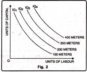
An Iso-product curve, on the other hand, represents a specific level of output. The level of output being a physical magnitude is measurable. We will therefore know the distance between two equal product curves. While indifference curves are labeled as IC1, IC2, IC3, etc., the Iso-product curves are labelled by the units of output they represent -100 metres, 200 metres, 300 metres of cloth then on.
Types of Iso-quant Curves
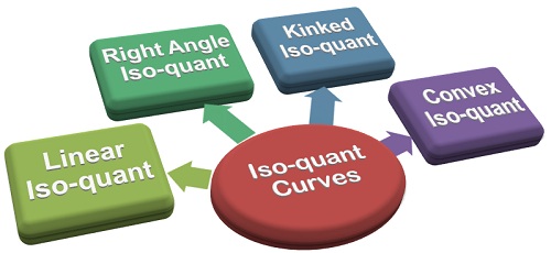
The Iso-quant curves are classified on the premise of the substitutability of factors of production. These are:
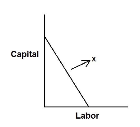
1. Linear Iso-quant Curve: This curve shows the perfect substitutability between the factors of production. This implies that any quantity is produced either employing only capital or only labor or through “n” number of combinations between these two.
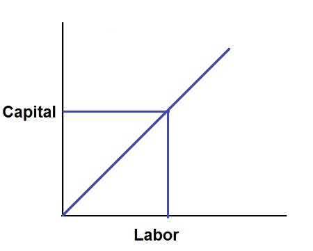
2. Right Angle Iso-quant Curve: this is one of the types of Iso-quant curves, where there's a strict complementarity with no substitution between the factors of production. According to this, there's only one method of production to produce any one commodity. This curve is also referred to as Leontief Iso-quant, input-output Isoquant and is a right angled curve.
3. Kinked Iso-quant Curve: This curve assumes, that there's a limited substitutability between the factors of production. This shows that substitution of factors is seen at the kinks since there are a few processes to produce any one commodity. Kinked Iso-quant curve is additionally referred to as activity analysis programming Iso-quant or linear programming Iso-quant.
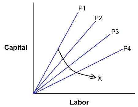
4. Convex Iso-quant Curve: In these sorts of Iso-quant curves, the factors are substituted for each other but up to a certain extent. This curve is smooth and convex to the origin.
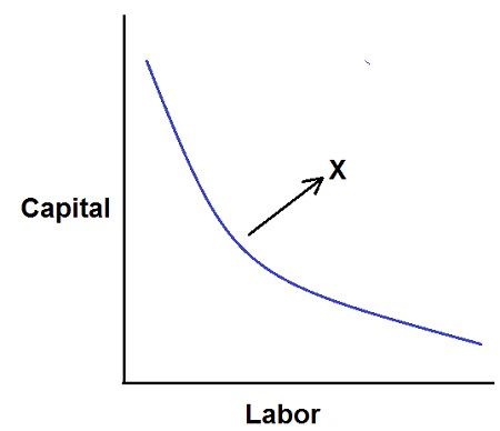
Thus, the classification of the Iso-quant curve is done on the premise of the number of labor units that can be substituted for capital and vice-versa, so on have the same level of production.
Properties of Iso-Product Curves:
The properties of Iso-product curves are summarized below:
1. Iso-Product Curves Slope Downward from Left to Right:
They slope downward because MTRS of labour for capital diminishes. When we increase labour, we've to decrease capital to produce a given level of output.
The downward sloping Iso-product curve is explained with the help of the subsequent figure:
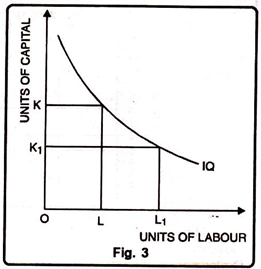
The Fig. 3 shows that when the amount of labour is increased from OL to OL1, the amount of capital must be decreased from ok to OK1, the Iso-product curve (IQ) is falling as shown in the figure.
The possibilities of horizontal, vertical, upward sloping curves is ruled out with the help of the subsequent figure 4:
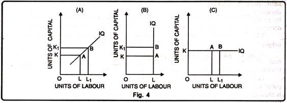
(i) The figure (A) shows that the amounts of both the factors of production are increased- labour from L to Li and capital from K to K1. When the amounts of both factors increase, the output must increase. Hence the IQ curve cannot slope upward from left to right.
(ii) The figure (B) shows that the amount of labour is kept constant while the amount of capital is increased. The amount of capital is increased from K to K1. Then the output must increase. So IQ curve can't be a vertical line.
(iii) The figure (C) shows a horizontal curve. If it's horizontal the number of labour increases, although the number of capital remains constant When the quantity of capital is increased, the extent of output must increase. Thus, an IQ curve can't be a horizontal line.
2. Isoquants are Convex to the Origin:
Like indifference curves, Isoquants are convex to the origin. So as to understand this fact, we've to understand the concept of diminishing marginal rate of technical substitution (MRTS), because convexity of an Isoquant implies that the MRTS diminishes along the Isoquant. The marginal rate of technical substitution between L and K is defined because the quantity of K which can be given up in exchange for an additional unit of L. It also can be defined as the slope of an Isoquant.
It is often expressed as:
MRTSLK = – ∆K/∆L = dK/ dL
Where ∆K is the change in capital and AL is the change in labour.
Equation (1) states that for an increase in the use of labour, fewer units of capital will be used. In other words, a declining MRTS refers to the falling marginal product of labour in relation to capital. To put it differently, as more units of labour are used, and as certain units of capital are given up, the marginal productivity of labour in relation to capital will decline.
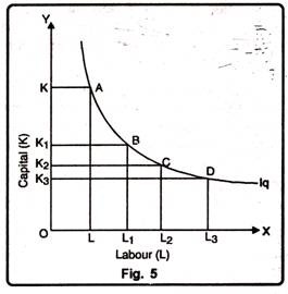
This fact can be explained in Fig. 5. As we move from point A to B, from B to C and from C to D along an Isoquant, the marginal rate of technical substitution (MRTS) of capital for labour diminishes. Every time labour units are increasing by an equal amount (AL) but the corresponding decreases in the units of capital (AK) decreases.
Thus it may be observed that because of falling MRTS, the Isoquant is always convex to the origin.
3. Two Iso-Product Curves Never Cut Each Other:
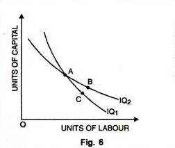
As two indifference curves cannot cut each other, two Iso-product curves cannot cut each other. In Fig. 6, two Iso-product curves intersect one another . Both curves IQ1 and IQ2 represent two levels of output. But they intersect one another at point A. Then combination A = B and combination A= C. Therefore B must be equal to C. This is often absurd. B and C lie on two different Iso-product curves. Therefore two curves which represent two levels of output cannot intersect one another.
4. Higher Iso-Product Curves Represent Higher Level of Output:
A higher Iso-product curve represents a higher level of output as shown within the figure 7 given below:
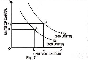
In the Fig. 7, units of labour have been taken on OX axis while on OY, units of capital. IQ1 represents an output level of 100 units whereas IQ2 represents 200 units of output.
5. Isoquants needn't be parallel to each Other:
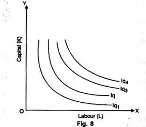
It so happens because the rate of substitution in different Isoquant schedules needn't be necessarily equal. Usually they're found different and, therefore, Isoquants may not be parallel as shown in Fig. 8. We may note that the Isoquants Iq1 and Iq2 are parallel but the Isoquants Iq3 and Iq4 aren't parallel to each other.
6. No Isoquant can Touch Either Axis:
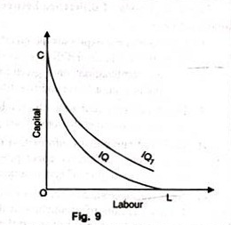
If an Isoquant touches X-axis, it would mean that the product is being produced with the help of labour alone without using capital at all. These logical absurdities for OL units of labour alone are unable to produce anything. Similarly, OC units of capital alone cannot produce anything without the utilization of labour. Therefore as seen in figure 9, IQ and IQ1 cannot be Isoquants.
An Isoquant represents combinations of two inputs that yield the same level of output. However, not all points of an Isoquant are relevant for production. Such points may be called infeasible points. One should consider only feasible portions of an Isoquant. This is often due to the fact that no rational producer will produce where marginal product of an input is either zero or negative.
If the Isoquant is backward bending and upward sloping, marginal product of any input are negative, and, hence, this portion of the Isoquant is also considered as economically non-sensible region of production. Only the negatively sloped segment of the Isoquant is relevant for production or economically feasible.
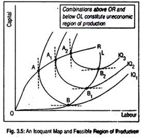
This is shown in Fig. 3.5 where we've drawn three Isoquants showing different levels of output for different labour-capital combinations. This diagram separates economic region of production from uneconomic region of production. Region in which marginal products of all inputs are positive constitutes economic region of production.
Or the region in which input substitution takes place is also called economic region of production. In an uneconomic region, as marginal product of an input becomes either zero or negative, the question of input substitution doesn't arise. Production in such region is, for obvious reasons, unprofitable or infeasible.
At point A on IQ1, the firm employs certain units of labour and capital. Since the tangent to IQ1 at point A is parallel to the vertical axis, marginal product of capital (MPK) is zero. If more capital is employed, marginal product of capital should be negative. In other words, beyond point A, MPK is negative. At point B on IQ1, MPL is zero and beyond point B on IQ1, MPL is negative.
Thus, points between A and B represent positive marginal productivities of both labour and capital. Here substitution between two inputs takes place. Similarly, points A1and A2 on IQ2 and IQ3 describe zero MPL while points beyond A1 and A2 describe negative MPK. Points B1and B2 on IQ2and IQ3 represent zero MPK and beyond B1 and B2 describe negative MPL.
A rational producer will produce in this region where marginal productivities of inputs are positive. By joining points A, A1 and A2 (i.e., points of zero marginal products) we get OR line and by joining points B, B1 and B2 (points of zero marginal products) we get OL line. These lines are called ridge lines. They provide the boundaries of the economic region of production where input substitution takes place.
Any point on the Isoquants outside the upper ridge line OR and therefore the lower ridge line OL constitute uneconomic region of production. Production must happen inside the ridge lines. Note that the ridge lines separate the relevant (i.e., negatively sloped) from the irrelevant portions (i.e., positively or zero sloped) of the Isoquants.
The firm may produce a particular quantity of its product at each of the alternative input combinations that lies on the IQ for that quantity. Since the firm’s goal is to maximise profit, the optimum input combination for producing a selected quantity of its product would be one that might produce the output at the minimum possible cost.
The optimum input combination in this case is understood as the least cost combination of inputs. So as to explain the firm’s selection of the least cost combination of inputs, let us suppose that a number of the firm’s Isoquants (IQs) and Iso-cost lines (ICLs) are given in Fig. 8.12.
Let us now suppose that the firm intends to produce a specific quantity q = q3 of its product, and therefore the Isoquant for this particular quantity is IQ3. In other words, if the firm uses any of the input combinations lying on IQ3, it would be able to produce the output quantity q = q3.
But, since the various points on IQ3, viz., S1, S2, S3, S4, S5, etc. lie on different ICLs, they produce the same output, viz., q = but at different levels of cost, For we all know that a higher (or a lower) ICL represents a higher (or a lower) level of cost.
Therefore, so as to produce the output of q3 at the least possible cost, the firm would need to select that point on IQ3 that would lie on the lowest possible ICL. In Fig. 8.12, we see that the point S3 on IQ3 lies on the lowest possible ICL, viz., L3M3. The other point on IQ3 lies on a higher ICL or a higher level of cost than L3M3.
Therefore, at an output of q3, the least cost combination of inputs is S3 (x̅, y̅). In other words, if the firm is to produce an output of q3, it would buy and use the quantity x of input X and therefore the quantity y of input Y. Here it's vital for us to observe that the least cost combination of inputs is that the point of tangency (here S3) between the particular Isoquant (here IQ3) and an Iso-cost line (here L3M3).
Similarly, for producing a specific quantity of output, if the firm is to remain on IQ2, then the least cost combination of inputs would run by the point T2, because this point is that the point of tangency between IQ2 and an ICL (i.e., L2M2).
Iso-Cost Line:
The Iso-cost line is similar to the price or budget line of the indifference curve analysis. It’s the line which shows the varied combinations of factors which will result in the same level of total cost. It refers to those different combinations of two factors that a firm can obtain at the same cost. Just as there are various Isoquant curves, so there are various Iso-cost lines, like different levels of total output.
Definition:
Iso-cost line is also defined as the line which shows different possible combinations of two factors that the producer can afford to buy given his total expenditure to be incurred on these factors and price of the factors.
Explanation:
The concept of Iso-cost line is explained with the help of the subsequent table 3 and Fig. 12. Suppose the producer’s budget for the acquisition of labour and capital is fixed at Rs. 100. Further suppose that a unit of labour cost the producer Rs. 10 while a unit of capital Rs. 20.

From the table cited above, the producer can adopt the subsequent options:
(i) Spending all the money on the acquisition of labour, he can hire 10 units of labour (100/10 = 10)
(ii) Spending all the money on the capital he may buy 5 units of capital.
(iii) Spending the money on both labour and capital, he can choose from various possible combinations of labour and capital like (4, 3) (2, 4) etc.
Diagram Representation:
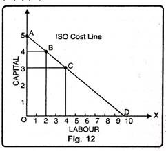
In Fig. 12, labour is given on OX-axis and capital on OY-axis. The points A, B, C and D convey the various combinations of two factors, capital and labour which can be purchased by spending Rs. 100. Point A indicates 5 units of capital and no unit of labour, while point D represents 10 units of labour and no unit of capital. Point B indicates 4 units of capital and 2 units of labour. Likewise, point C represents 4 units of labour and three units of capital.
Iso-Cost Curves:
After knowing the character of Isoquants which represent the output possibilities of a firm from a given combination of two inputs We further extend it to the prices of the inputs as represented on the Isoquant map by the Iso-cost curves.
These curves are referred to as outlay lines, price lines, input-price lines, factor-cost lines, constant-outlay lines, etc. Each Iso-cost curve represents the various combinations of two inputs that a firm can buy for a given sum of money at the given price of each input.
Figure 13 (A) shows three Iso-cost curves each represents a total outlay of 50, 75 and 100 respectively. The firm can hire OC of capital or OD of labour with Rs. 75. OC is 2/3 of OD which implies that the price of a unit of labour is 1/2 times but that of a unit of capital.
The line CD represents the price ratio of capital and labour. Prices of factors remaining the same, if the total outlay is raised, the Iso-cost curve will shift upward to the right as EF parallel to CD, and if the total outlay is reduced it'll shift downwards to the left as AB
The Iso-costs are straight lines because factor prices remain the same regardless of the outlay of the firm on the two factors.
The Iso-cost curves represent the locus of all combinations of the two input factors which lead to the same total cost. If the unit cost of labour (L) is w and therefore the unit cost of capital (C) is r, then the total cost: TC = wL + rC. The slope of the Iso-cost line is that the ratio of prices of labour and capital i.e., w/r.
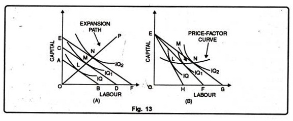
The point where the Iso-cost line is tangent to an Isoquant shows the least cost combination of the 2 factors for producing a given output. If all points of tangency like LMN are joined by a line, it's referred to as an output-factor curve or least-outlay curve or the expansion path of a firm.
It shows how the proportions of the 2 factors used could be changed as the firm expands. Forinstance, in Figure 13 (A) the proportions of capital and labour wont to produce 200 (IQ1) units of the product are different from the proportions of those factors used to produce 300 (IQ2) units or 100 units at the lowest cost.
Like the price-income line in the indifference curve analysis, a relative cheapening of 1 of the factors to that of another will extend the Iso-cost line to the right. If one of the factors becomes relatively dearer, the Iso-cost line will contract inward to the left.
Given the price of capital, if the price of labour falls, the Isocost line EF in Panel (B) of figure 13 will extend to the right as EG and if the price of labour rises, the Iso-cost line EF will contract inward to the left as EH, if the equilibrium points L, M, and N are joined by a line. It’ll be called the price-factor curve.
We know that the production function of the firm
q = f(x,y) (8.21)
Gives us the Isoquant map of the firm, one Isoquant (IQ) for each particular level of output, and also the cost equation of the firm
C = rXx + rYy (8.54)
Gives us the family of parallel Iso-cost lines (ICLs), given the prices of the inputs rX and rY, one ICL for one particular level of cost. The IQ-map and therefore the family of ICLs are given in Fig. 8.14. If we now join the point of origin 0 and therefore the points of tangency, E1, E2, E3, etc., between the IQs and therefore the ICLs by a curve, then this curve (OK in Fig. 8.14) would give us what is called the expansion path of the firm.
The expansion path is so called because if the firm decides to expand its operations, it might need to move along this path. Allow us to note that the firm may expand in two ways.
First, it's going to want to expand by successively increasing its level of cost or its expenditure on the inputs X and Y, i.e., by using more and more of inputs, and, consequently, by producing more of its output.
Second, the firm may plan to expand by increasing its level of output per period. This the firm may do by increasing the expenditure on the inputs, i.e., by using more and more of them.
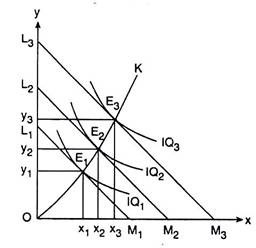
Fig.8. 14 The expansion path of a firm
The two approaches to expansion apparently appear to be the same, for both involve an increase in expenditure. However, there's a fundamental difference. In the first case, decision is taken initially at the point of cost. Cost levels are made higher and higher then efforts are made to maximise the level of output subject to the cost constraint.
On the opposite hand, within the second case, decision-making occurs initially and directly at the point of output. Here the firm first decides to produce more of output then efforts are made to produce the output at the minimum possible cost.
(a) Expansion by Means of increasing the level of Expenditure on the Inputs:
In Fig. 8.14, allow us to suppose that, initially, the firm’s level of cost is such its ICL is L1M1 and output-maximisation subject to cost constraint occurs at the point of tangency, E1, between the ICL, L1M1, and an IQ which is IQ1. At E1 the firm uses X1 of the first input and y1 of the second input to produce the maximum possible output, say, q1, which is represented by IQ1.
Now, if the firm decides to expand by increasing the cost level from the level of L1M1 to that of L2M2, then the firm would be in output-maximising equilibrium at the point of tangency E2 (x2, y2), on IQ2, using more of the inputs, x2 > x1 and y2 > y1, and producing an output level, say, q2, q2 > q1, since IQ2 is a higher Isoquant than IQ1.
In the same way, if the firm decides to expand further, it might increase its cost level from that of L2M2 to that of L3M3 and it might produce the maximum output subject to the cost constraint at the point of tangency E3 (x3, y3) on IQ3 using more of the inputs, x3 > x2 and y3 > y2, and producing a higher level of output, say, q3, q3 > q2, since IQ3 is a higher IQ than IQ2.
The process of expansion of firm’s operations through increases in the level of cost may go on in this say so long because the firm decides in its favour. If we now join the point of origin O and therefore the points E1, E2, E3, etc. by a path, and then we would obtain the firm’s expansion path OK in Fig. 8.14.
That is, if the firm expands by increasing its level of cost, it might have to move successively from one equilibrium point to another along this expansion path.
We have joined the path through the equilibrium points E1, E2, etc. with the point of origin O, because if the firm moves backward along the expansion path by decreasing the cost level then it might be moving from the initial equilibrium point, say, E3 to E2, then from E2 to E) and would approach the point O which would be the limiting point in this process.
As the firm’s cost level decreases and tends to zero, the input quantities and therefore the output quantity would all decrease and tend to zero, and thus the point of origin O would be the limiting point.
(b) Expansion by Means of increasing the level of Output:
In Fig. 8.14, allow us to suppose that initially the firm decides to produce q1 of output which may be produced at any point on the Isoquant, IQ1. The firm would be in cost-minimising equilibrium at the point E1 which is that the point of tangency between IQ1 and an Iso-cost line say, ICL1. At the point E1, the firm would use Xi and y] quantities of the 2 inputs and its cost amounts to, say, C1, which is that the minimum possible.
The firm may now plan to expand by increasing its level of output from q1 to q2 on IQ2. If the firm makes this decision, its cost-minimising equilibrium are obtained at the point of tangency E2 (x2, y2) on L2M2 using more of the inputs, x2 > x1 and y2 > y1 and incurring a cost level C2 on L2M2, which is that the minimum possible required to produce the output of q2. However, C2 > C1 since L2M2 is a higher ICL than L2M2.
The firm’s process of expansion may go on like this as long as it decides to expand. The expansion path again would be OK that might start from the point of origin O and pass through the points E1, E2, E3, etc.
If the firm decides to contract and produce less of output, then the limiting point of the process of contraction would be the point of origin O, where the firm’s use of the inputs, its cost level and output would all tend to zero.
Meaning:
Law of variable proportions occupies a vital place in economic theory. This law examines the production function with one factor variable, keeping the quantities of other factors fixed. In other words, it refers to the input-output relation when output is increased by varying the quantity of 1 input.
When the quantity of 1 factor is varied, keeping the quantity of other factors con¬stant, the proportion between the variable factor and therefore the fixed factor is altered; the ratio of employment of the variable factor to that of the fixed factor goes on increasing because the quantity of the variable factor is increased.
Since under this law we study the effects on output of variation in factor proportions, this is often also referred to as the law of variable proportions. Thus law of variable proportions is the new name for the famous “Law of Diminishing Returns” of classical economics. This law has played an important role in the history of economic thought and occupies an equally important place in modern economic theory. This law has been supported by the empirical evidence about the real world.
The law of variable proportions or diminishing returns has been stated by various economists within the following manner:
As equal increments of 1 input are added; the inputs of other productive services being held constant, beyond a particular point the resulting increments of product will decrease, i.e., the marginal products will diminish,” (G. Stigler)
“As the proportion of 1 factor in a combination of factors is increased, after some extent , first the marginal and then the average product of that factor will diminish.” (F. Benham)
“An increase in some inputs relative to other fixed inputs will, in a given state of technology, cause output to increase; but after a point the extra output resulting from the same addition of extra inputs will become less.” (Paul A. Samuelson)
Marshall discussed the law of diminishing returns in reference to agriculture. He defines the law as follows: “An increase in the capital and labour applied within the cultivation of land causes generally a less than proportionate increase in the amount of product raised unless it happens to coincide with an improvement in the arts of agriculture.”
It is obvious from the above definitions of the law of variable proportions (or the law of diminishing returns) that it refers to the behaviour of output because the quantity of 1 factor is increased, keeping the quantity of other factors fixed and further it states that the marginal product and average product will eventually decline.
Assumptions of the Law:
The law of variable proportions or diminishing returns, as stated above, holds good under the subsequent conditions:
1. First, the state of technology is assumed to be given and unchanged. If there's improvement in the technology, then marginal and average products may rise rather than diminishing.
2. Secondly, there must be some inputs whose quantity is kept fixed. This is often one of the ways by which we will alter the factor proportions and know its effect on output. This law doesn't apply in case all factors are proportionately varied. Behaviour of output as results of the variation in all inputs is discussed under “returns to scale”.
3. Thirdly the law is predicated upon the possibility of varying the proportions in which the varied factors can be combined to produce a product. The law doesn't apply to those cases where the factors must be utilized in fixed proportions to yield a product.
When the varied factors are required to be utilized in rigidly fixed proportions, then the increase in one factor wouldn't lead to any increase in output, that is, the marginal product of the factor will then be zero and not diminishing. It may, however, be pointed out that products requiring fixed proportions of factors are quiet uncommon. Thus, the law of variable proportion applies to most of the cases of production in the real world.
The law of variable proportions is illustrated in Table 16.1.and Fig. 16.3. We shall first explain it by considering Table 16.1. Assume that there's a given fixed amount of land, with which more units of the variable factor labour, is employed to produce agricultural output.
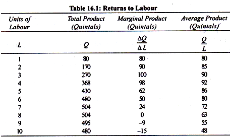
With a given fixed quantity of land, as a farmer raises employment of labour from one unit to 7 units, the total product increases from 80 quintals to 504 quintals of wheat. Beyond the employment of 8 units of labour, total product diminishes. It's worth noting that up to the utilization of three units of labour, total product increases at an increasing rate.
This fact is clearly revealed from column 3 which shows successive marginal prod¬ucts of labour as extra units of labour are used. Marginal product of labour, it's going to be recalled, is that the increment in total output due to the utilization of an extra unit of labour.
It will be seen from Col. 3 of Table 16.1, that the marginal product of labour initially rises and beyond the utilization of three units of labour, it starts diminishing. Thus when 3 units of labour are employed, marginal product of labour is 100 and with the utilization of 4th and 5th units of labour marginal product of labour falls to 98 and 62 respectively.
Beyond the utilization of eight units of labour, total product diminishes and thus marginal product of labour becomes negative. As regards average product of labour, it rises up to the utilization of fourth unit of labour and beyond that it's falling throughout.
Three Stages of the Law of Variable Proportions:
The behaviour of output when the varying quantity of 1 factor is combined with a fixed quantity of the other are often divided into three distinct stages. So as to know these three stages it's better to graphically illustrate the production function with one factor variable.
This has been done in Fig. 16.3. In this figure, on the X-axis the quantity of the variable factor is measured and on the F-axis the total product, average product and marginal product are measured. How the total product, average product and marginal product a variable factor change as a results of the increase in its quantity, that is, by increasing the quantity of 1 factor to a fixed quantity of the others are going to be seen from Fig. 16.3.
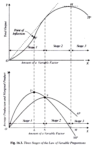
In the top Danel of this figure, the total product curve TP of variable factor goes on increasing to a point and alter that it starts declining. In the bottom pane- average and marginal product curves of labour also rise then decline; marginal product curve starts declining before the average product curve.
The behaviour of these total, average and marginal products of the variable factor as results of the rise in its amount is mostly divided into three stages which are explained below:
Stage 1:
In this stage, total product curve TP increases at an increasing rate up to a point. In Fig. 16.3. From the origin to the point F, slope of the total product curve TP is increasing, that is, up to the point F, the total product increases at an increasing rate (the total product curve TP is concave upward up to the point F), which suggests that the marginal product MP of the variable factor is rising.
From the point F onwards during the stage 1, the total product curve goes on rising but its slope is declining which suggests that from point F onwards the total product increases at a diminishing rate (total product curve TP is concave down-ward), i.e., marginal product falls but is positive.
The point F where the total product stops increasing at an increasing rate and starts increasing at the diminishing rate is named the point of inflection. Vertically corresponding to the current point of inflection marginal product is maximum, after which it starts diminishing.
Thus, marginal product of the variable factor starts diminishing beyond OL amount of the variable factor. That is, law of diminishing returns starts operating in stage 1 from point D on the MP curve or from OL amount of the variable factor used.
This first stage ends where the average product curve AP reaches its highest point, that is, point S on AP curve or CW amount of the variable factor used. During stage 1, when marginal product of the variable factor is falling it still exceeds its average product then continues to cause the average product curve to rise.
Thus, during stage 1, whereas marginal product curve of a variable factor rises during a part then falls, the average product curve rises throughout. In the first stage, the quantity of the fixed factor is too much relative to the quantity of the variable factor so if some of the fixed factor is withdrawn, the total product will increase. Thus, within the first stage marginal product of the fixed factor is negative.
Stage 2:
In stage 2, the total product continues to increase at a diminishing rate until it reaches its maximum point H where the second stage ends. In this stage both the marginal product and therefore the average product of the variable factor are diminishing but remain positive.
At the end of the second stage, that is, at point M marginal product of the variable factor is zero (corresponding to the highest point H of the total product curve TP). Stage 2 is extremely crucial and important because as are going to be explained below the firm will seek to produce in its range.
Stage 3: Stage of Negative Returns:
In stage 3 with the rise in the variable factor the total product declines and thus the total product curve TP slopes downward. As a result, marginal product of the variable factor is negative and therefore the marginal product curve MP goes below the X-axis. During this stage the variable factor is too much relative to the fixed factor. This stage is named the stage of negative returns, since the marginal product of the variable factor is negative during this stage.
It may be noted that stage 1 and stage 3 are completely symmetrical. In stage 1 the fixed factor is too much relative to the variable factor. Therefore, in stage 1, marginal product of the fixed factor is negative. On the opposite hand, in stage 3 the variable factor is too much relative to the fixed factor. Therefore, in stage 3, the marginal product of the variable factor is negative.
The Stage of Operation:
Now, a very important question is in which stage a rational producer will seek to produce. A rational producer will never prefer to produce in stage 3 where marginal product of the variable factor is negative. Marginal product of the variable factor being negative in stage 3, a producer can always increase his output by reducing the amount of the variable factor.
It is thus clear that a rational producer will never be producing in stage 3. Even if the variable factor is free, the rational producer will stop at the end of the second stage where the marginal product of the variable factor is zero.
At the end point M of the second stage where the marginal product of the variable factor is zero, the producer are going to be maximising the total product and will thus be making maximum use of the variable factor. A rational producer also will not prefer to produce in stage 1 where the marginal product of the fixed factor is negative.
A producer producing in stage 1 means he will not be making the best use of the fixed factor and further that he won't be utilising fully the opportunities of increasing production by increasing quantity of the variable factor whose average product continues to rise throughout the stage 1. Thus, a rational entrepreneur will not stop in stage 1 but will expand further.
Even if the fixed factor is free (i.e., costs nothing), the rational entrepreneur will stop only at the end of stage 1 (i.e., at point N) where the average product of the variable factor is maximum. At the end point N of stage 1, the producer they're going to be making maximum use of the fixed factor.
It is thus clear from above that the rational producer will never be found producing in stage 1 and stage 3. Stage 1 and three may, therefore, be called stages of economic absurdity or economic non-sense. The stages 1 and three represent non-economic regions in production function.
A rational producer will always seek to produce in stage 2 where both the marginal product and average product of the variable factor are diminishing. At which particular point during this stage, the producer will plan to produce depends upon the prices of factors. The stage 2 represents the range of rational production decisions.
We have seen above how output varies as the factor proportions are altered at any given moment. We have also noticed that this input-output relation can be divided into three stages. Now, the question arises on what causes increasing marginal returns to the variable factor in the start, diminishing marginal returns later and negative marginal returns to the variable factor ultimately.
Causes of Initial Increasing marginal Returns to a Factor:
In the beginning, the number of the fixed factor is abundant relative to the number of the variable factor. Therefore, when more and more units of a variable factor are added to the constant quantity of the fixed factor, the fixed factor is more intensively and effectively utilised.
This causes the production to rise at a rapid rate. When, in the beginning the variable factor is comparatively smaller in quantity, some amount of the fixed factor may remain unutilised and thus when the variable factor is increased fuller utilisation of the fixed factor becomes possible with the result that increasing returns are obtained.
The question arises as to why the fixed factor isn't initially taken in an appropriate quantity which suits the available quantity of the variable factor. Answer to the present question is provided by the fact that generally those factors are taken as fixed which are indivisible. Indivisibility of a factor means that because of technological requirements a minimum amount of that factor must be used whatever the level of output.
Thus, as more units of variable factor are employed to figure with an indivisible fixed factor, output greatly increases within the beginning due to fuller and more effective utilisation of the latter. Thus, we see that it's the indivisibility of some factors which causes increasing returns to the variable factor in the start .
The second reason why we get increasing returns to the variable factor in the initial stage is that as more units of the variable factor are employed the efficiency of the variable factor itself increases. This is often because when there's a sufficient quantity of the variable factor, it becomes possible to introduce specialisation or division of labour which results in higher productivity. The greater the quantity of the variable factor, the greater the scope of specialisation and hence the greater will be the level of its productivity or efficiency.
Causes of Diminishing marginal Returns to a Factor:
The stage of diminishing marginal returns in the production function with one factor variable is the most significant. The question arises as to why we get diminishing marginal returns after a particular amount of the variable factor has been added to a fixed quantity of the opposite factor.
As explained above, increasing returns to a variable factor occur initially primarily as a result of the more effective and fuller use of the fixed factor becomes possible as more units of the variable factor are employed to work with it.
Once the point is reached at which the quantity of the variable factor is sufficient to ensure the efficient utilisation of the fixed factor, then further increases within the variable factor will cause marginal and average products of a variable factor to decline because the fixed factor then becomes inadequate relative to the number of the variable factor.
In other words, the contributions to the production made by the variable factor after a point become less and less because the extra units of the variable factor have less and less of the fixed factor to work with. The production is that the results of the co-operation of varied factors aiding each other. Now, how much aid one factor provides to the others depends upon how much there's of it.
Eventually, the fixed factor is abundant relative to the amount of the variable factor and the former provides much aid to the later. Eventually, the fixed factor becomes more and more scarce in reference to the variable factor so that as the units of the variable factor are increased they receive less and less aid from the fixed factor. As a result, the marginal and average products of the variable factor decline ultimately.
The phenomenon of diminishing marginal returns, like that of increasing marginal returns, rests upon the indivisibility of the fixed factor. As explained above, the important reason for increasing returns to a factor within the beginning is that the fact that the fixed factor is indivisible which has got to be employed whether the output to be produced is small or large.
When the indivisible fixed factor isn't being fully used, successive increases in a variable factor add more to output since fuller and more efficient use is formed of the indivisible fixed factor. But there's generally a limit to the range of employment of the variable factor over which its marginal and average products will increase.
There will usually be a level of employment of the Variable factor at which indivisible fixed factor is being as fully and efficiently used as possible. It’ll happen when the variable factor has increased to such an amount that the fixed indivisible factor is getting used in the “best or optimum proportion” with the variable factor.
Once the optimum proportion is disturbed by further increases within the variable factor, returns to a variable factor (i.e., marginal product and average product) will diminish primarily because the indivisible factor is getting used too intensively, or in other words, the fixed factor is getting used in non-optimal proportion with the variable factor.
Just as the marginal product of the variable factor increases within the first stage when better and fuller use of the fixed indivisible factor is being made, therefore the marginal product of the variable factor diminishes when the fixed indivisible factor is being worked too hard.
If the fixed factor was perfectly divisible, neither the increasing nor the diminishing returns to a variable factor would have occurred. If the factors were perfectly divisible, then there wouldn't are the need of taking a large quantity of the fixed factor in the start to combine with the varying quantities of the opposite factor.
In the presence of perfect divisibility, the optimum proportion between the factors could have always been achieved. Perfect divisibility of the factors implies that a small firm with a small machine and one worker would be as efficient as a large firm with a large machine and lots of workers.
The productivity of the factors would be the same in the two cases. Thus, we see that if the factors were perfectly divisible, then the question of varying factor proportions wouldn't have arisen and hence the phenomena of increasing and diminishing marginal returns to a variable factor wouldn't have occurred. Prof. Bober rightly remarks: “Let divisibility enter through the door, law of variable proportions rushes out through the window.”
Joan Robinson goes deeper into the causes of diminishing returns. She holds that the diminishing marginal returns occur because the factors of production are imperfect substitutes for each other. As seen above, diminishing returns occur during the second stage since the fixed factor is now inadequate relatively to the variable factor. Now, a factor which is scarce in supply is taken as fixed.
When there's a scarce factor, quantity of that factor cannot be increased in accordance with the varying quantities of the opposite factors, which, after the optimum proportion of factors is achieved, leads to diminishing returns.
If now some factors were available which perfect substitute of the scarce fixed factor was, then the paucity of the scarce fixed factor during the second stage would are made up by the increase in supply of its perfect substitute with the result that output could be expanded without diminishing returns.
Thus, even if one of the variable factors which we add to the fixed factor were perfect substitute of the fixed factor, then when, in the second stage, the fixed factor becomes relatively deficient; its deficiency would have been made up the increase in the variable factor which is its perfect substitute.
Thus, Joan Robinson says, “What the Law of Diminishing Returns really states is that there's a limit to the extent to which one factor of production is substituted for an additional , or, in other words, that the elasticity of substitution between factor isn't infinite.
If this were not true, it might be possible, when one factor of production is fixed in amount and therefore the rest are in perfectly elastic supply, to produce a part of the output with the help of the fixed factor, and then, when the optimum proportion between this and other factors was attained, to substitute another factor for it and to increase output at constant cost.” We, therefore, see that diminishing returns operate because the elasticity of substitution between factors isn't infinite.
Explanation of Negative Marginal Returns to a Factor:
As the amount of a variable factor continues to be increased to a fixed quantity of the other factor, a stage is reached when the total product declines and therefore the marginal product of the variable factor becomes negative.
This phenomenon of negative marginal returns to the variable think about stage 3 is because of the fact that the amount of the variable factor becomes too excessive relative to the fixed factor so they obstruct one another with the result that the total output falls rather than rising.
Besides, large a number of the variable factor also impairs the efficiency of the fixed factor. The proverb “too many cooks spoil the broth” aptly applies to the present situation. In such a situation, a reduction within the units of the variable factor will increase the total output.
The laws of returns to scale also can be explained in terms of the Isoquant approach. The laws of returns to scale refer to the results of a change within the scale of factors (inputs) upon output within the long run when the combinations of factors are changed within the same proportion.
If by increasing two factors, say labour and capital, within the same proportion, output increases in just the same proportion, there are constant returns to scale. If so as to secure equal increases in output, both factors are increased in larger proportionate units, there are decreasing returns to scale. If so as to get equal increases in output, both factors are increased in smaller proportionate units, there are increasing returns to scale.
The returns to scale are often shown diagrammatically on an expansion path “by the gap between successive ‘multiple-level-of-output” Isoquants, that is, Isoquants that show levels of output which are multiples of some base level of output, e.g., 100, 200, 300, etc.”
Increasing Returns to Scale:
Figure 8 shows the case of increasing returns to scale where to urge equal increases in output, lesser proportionate increases in both factors, labour and capital, are required.
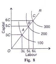
It follows that within the figure:
100 units of output require 3C + 3L
200 units of output require 5C + 5L
300 units of output require 6C + 6L
So that along the expansion path OR, OA > AB > BC. In this case, the production function is homogeneous of degree greater than one. The increasing returns to scale are attributed to the existence of indivisibilities in machines, management, labour, finance, etc. Some items of apparatus or some activities have a minimum size and cannot be divided into smaller units. When a business unit expands, the returns to scale increase because the indivisible factors are employed to their full capacity
Increasing returns to scale also result from specialisation and division of labour. When the scale of the firm expands there's wide scope for specialisation and division of labour. Work is divided into small tasks and workers will be concentrated to narrower range of processes. For this, specialized equipment is installed.
Thus with specialization efficiency increases and increasing returns to scale follow:
Further, because the firm expands, it enjoys internal economies of production. It's going to be able to install better machines, sell its products more easily, borrow money cheaply, procure the services of more efficient manager and workers, etc. of these economies help in increasing the returns to scale quite proportionately.
Not only this, a firm also enjoys increasing returns to scale because of external economies. When the industry itself expands to satisfy the increased long-run demand for its product, external economies appear which are shared by all the firms within the industry. When a large number of firms are concentrated at one place, skilled labour, credit and transport facilities are easily available.
Subsidiary industries occur to assist the main industry. Trade journals, research and training centres appear which help in increasing the productive efficiency of the firms. Thus these external economies also are the reason for increasing returns to scale.
Decreasing Returns to Scale:
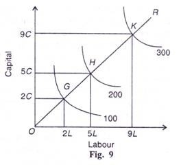
Figure 9 shows the case of decreasing returns where to urge equal increases in output, larger proportionate increases in both labour and capital are required.
It follows that:
100 units of output require 2C + 2L
200 units of output require 5C + 5L
300 units of output require 9C + 9L
So that along the expansion path OR, OG < GH < HK.
In this case, the production function is homogeneous of degree but one. Returns to scale may start diminishing because of the subsequent factors. Indivisible factors may become inefficient and less productive. Business may become unwieldy and produce problems of supervision and coordination.
Large management creates difficulties of control and rigidities. To those internal diseconomies are added external diseconomies of scale. These arise from higher factor prices or from diminishing productivities of the factors. Because the industry continues to expand the demand for skilled labour, land, capital, etc. rises.
There being perfect competition, intensive bidding raises wages, rent and interest. Prices of raw materials also go up. Transport and marketing difficulties emerge. Of these factors tend to lift costs and therefore the expansion of the firms results in diminishing returns to scale so that doubling the scale wouldn't result in doubling the output.
Constant Returns to Scale:
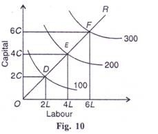
Figure 10 shows the case of constant returns to scale. Where the distance between the Isoquants 100, 200 and 300 along the expansion path OR is that the same, i.e., OD = DE = EF. It implies that if units of both factors, labour and capital, are doubled, the output is doubled. To treble the output, units of both factors are trebled.
It follows that:
100 units of output require
1 (2C + 2L) = 2C + 2L
200 units of output require
2 (2C + 2L) = 4C + 4L
300 units of output require
3 (2C + 2L) = 6C + 6L
The returns to scale are constant when internal economies enjoyed by a firm are neutralised by internal diseconomies in order that output increases within the same proportion. One more reason is the balancing of external economies and external diseconomies.
Constant returns to scale also result when factors of production are perfectly divisible, substitutable, and homogeneous and their supplies are perfectly elastic at given prices. That’s why, within the case of constant returns to scale, the production function is homogeneous of degree one.
According to Alfred Marshall Economies of scale are broadly classified into internal economies of scale and external economies of scale. In the large-scale production, the cost of production should be low which is named as economies of scale. A firm enjoy internal economies of scale when he expands his size or scale of production in economy by making changes within the internal factors of production. Where on the other hand a firm enjoy internal economies of scale when he expands his size of production ineconomy by making changes within the external factors of production
INTERNAL ECONOMIES OF SCALE
Internal economies of scale are an increase within the scale or size of production or output of a firm these are solely enjoyable by firm independently by making changes within the input factors of production into his business. The internal economies of scale have various differing kinds which are as follows:
1) Labour economies: Adam Smith in this book “An inquiry into the nature and causes of the wealth of the nation” 1776 emphasised on the division of labour. Economies of labour also imply the benefit which is arising within the scale of economy because of division of labour. Division of labour increases the efficiency in production which results in increase within the size of output. Division of labour bring specialisation in labour skills and also saves time which successively increases the level or scale of output. Thus, with the specialisation of division of labour the firm produces large scale of production.
2) Technical economies: technique of production also increases the scale of production. In other words, technical economies refer to increase within the scale of production because of change in technical or methods of production which reduces the cost of production.
Technical economies increase the dimension of firms where the average cost of production decreases and average revenue are going to be high.
3) Managerial economies: Manager plays an important role in managing business activities. Managerial economies refer to the specialisation of managerial function which increases the extent of output. It’s a mangers duty to carry out all the managerial decision efficiently and effectively within the business enterprise. Division of managerial activities increases the management of the business efficiently.
4) Financial economies: finance plays and important role in process of production. It's one among the important and essential factors of production. It's always observed that the large firms enjoy the advantage of better credit facility from banks then the small scale firm. They also get the credit quickly and simply then the small firm or producer.
5) Marketing economies: marketing economies deals with the process of buying raw materials and selling of finished goods. A large firm have a good bargaining power. By using firm raw material at cheaper cost as it buys in bulk then the small firm. This successively helps him to produce more at less cost and sell large amount of output within the market than the small firm.
6) Transport and storage: The large-scale firm have its own transport and storage facility which reduces his transportation and storage cost. This reduces the average cost of large-scale firm and increase the size of output or revenue. Where the small-scale firms hire or pay rent for the utilization of transport and storage facility.
EXTERNAL ECONOMIES OF SCALE
External economies of scale refer to those economies which provide benefits and facilities to all firms of given industry. It is an economy which is enjoyed by all firms of industry regardless of their size of operation. External economies of scale also are of various types which are follows:
1) Localisation economies: when variety of firms are located on one place with an objective of deriving the mutual benefits of training of skilled labour, provision of better transport facility etc. all these advantage helps the firm to cut back cost of production. Thus, localisation economies refer to concentration of a specific industry in one area which ends up in the development of conditions of industry which can reap the mutual benefits of all firms in the economy.
2) Disintegration economies: disintegration means firms splitting up its operation and therefore the process of manufacture and handing over the specialised agency and institution is named economies of disintegration. There are two sorts of disintegration like vertical and horizontal disintegration of economies. The firm which operates on disintegration of economies of scale are able to get economies of scale when it operates on a large scale.
3) Information economies: proper information in economy plays an important role for the producer to grow his economy. Networking with one another enables firms to make marketing and technical information easily
4) By-product economies: to manufacture by-products a largescalefirm make use of waste material. This may help the entire firm in the industry to reduce the waste within the economy and make efficient use of resources. This may ultimately reduce the cost of production and increase the extent of output.
Types of Internal Economies:
Internal economies which arise from the expansion of a firm are the following:
(1) Technical Economies:
Technical economies are those which arise to a firm from the utilization of better machines and techniques of production. As a result, production increases and therefore the per unit cost of production falls. Prof. Cairncross divides technical economies into the subsequent five parts:
(i) Economies of Superior Technique:
It is only large firms which may afford to buy costly machines and install them. Such machines are more productive than small machines. The high cost of such machines are often spread over a larger output which they help to produce. Thus the per unit cost of production falls in a very large firm which employs costly and superior plant and equipment and thereby enjoys a technical superiority over a small firm.
(ii) Economies of Increased Dimensions:
The installation of large machines itself brings many advantages to a firm. The cost of operating large machines is a smaller amount than that of operating small machines. Even the cost of construction is comparatively lower for giant machines than for small ones. The manufacture of a double- Decker bus is lower as compared to the manufacture of two ordinary buses. Moreover, a double-decker carries more passengers than a standard bus and at the same time requires only a driver and a conductor just like the latter. Thus its operating costs are relatively lower.
(iii) Economies of Linked Processes:
A large firm is in a position to reduce its per unit cost of production by linking the varied processes of production. As an example , a large sugar manufacturing firm may own its sugarcane farms, manufacture sugar, pack it in bags, transport and distribute sugar through its own transport and distribution departments. Thus by linking the varied processes of production and sale, a large firm saves the expenses incurred on intermediaries, thereby reducing unit cost of production.
(iv) Economies of the use of By-Products:
A large firm possesses greater resources than a small firm and is in a position to utilise its waste material as a by-product. For instance , the molasses left over after manufacturing sugar from the sugarcane are often used for producing spirit by installing a plant for the purpose.
(v) Economies of Increased Specialisation:
A large firm is in a position to reap economies by dividing its production processes into sub-processes thereby resulting in greater division of labour and to increased specialisation. This increases the productive efficiency of the firm and reduces the unit cost of production.
(2) Marketing Economies:
A large firm also reaps the economies of buying and selling. It buys its requirements of varied inputs in bulk and is, therefore, able to secure them at favourable terms in the sort of better quality inputs, prompt delivery, transport concessions, etc. due to its larger organisation, it produces quality products which are offered for sale in attractive packing by its packing department. It may also have a sales department manned by experts who carry on salesmanship, propaganda and advertisement through the varied media efficiently. Thus a large firm is in a position to reap the economies of marketing through its superior bargaining power and efficient packing and sales organisation.
(3) Managerial Economies:
A large firm can afford to put specialists to supervise and manage the varied departments. There is also a separate head for manufacturing, assembling, packing, marketing, general administration, etc. This results in functional specialisation which increases the productive efficiency of the firm. These managerial economies also reduce per unit cost of management because with expansion of the firm, the varied departmental managers will manage large output as efficiently as they were managing small output at the same salary.
(4) Financial Economies:
A large firm can procure cheap and timely finance both from the banks and therefore the market because it possesses large assets and good reputation. It also can raise fresh capital by floating shares and debentures within the capital market. It's during this way that a large firm reaps financial economies.
(5) Risk-Bearing Economies:
A large firm is in a better position than a small firm in spreading its risks. It can produce a range of products, and sell them in several areas. By the diversification, of its products the big firm is in a position to reduce risks by counter-balancing the loss of 1 product by the gain from other products. By the diversification of markets, it can counter-balance the autumn in demand in one market by the increased demand in other markets. Albeit the demand within the other markets for the products of the firm is constant, the loss are often easily borne by it.
A firm undertakes great risk by depending excessively on one source for its supply of power and raw materials. It can avoid risks by having alternative sources of supply within the case of power and different sources for the availability of raw materials. As an example , a large firm can avoid the losses arising from failure of regular power-supply by installing a generator of its own.
(6) Economies of Research:
A large firm possesses-larger resources than a small firm and may establish its own research laboratory and use trained research workers. Once they invent new production techniques or processes, the latter become the property of the firm which utilises them for increasing its output and reducing costs.
(7) Economies of Welfare:
All firms need to provide welfare facilities to their workers. But a large firm, with its large resources, can provide better working conditions in and outside the factory. It's going to run subsidised canteens, provide crèches for the infants of women workers and recreation rooms for the workers within the factory premises. It’s going to also provide cheap houses, educational and medical facilities for the families of workers and recreational clubs outside the factory. Though the expenses on such facilities are very heavy, yet they have a tendency to increase the productive efficiency of the workers which helps in raising production and reducing costs.
(B) External Economies:
External economies benefit all firms within the industry because the size of the industry expands. Such economies accrue to firms when the industry is localised during a particular area, makes inventions and evolves specialisation of production processes. These external economies are discussed below.
(1) Economies of Concentration:
When an industry is concentrated during a particular area, all the member firms reap some common economies. First, skilled labour is obtainable to all the firms. Second, means of transport and communications are considerably improved. The industry may ask the railway authorities for extra facilities for more wagons, loading and unloading, etc. Road transporters can also provide special facilities to the firms. Third, banks, insurance companies and other financial institutions set up their offices within the area and therefore the firms get cheap and timely credit. Fourth, the electricity board supplies adequate power to the firms, often at concessional rates. Lost, subsidiary industries develop to supply the localised industry with tools, equipment and raw materials. Of these facilities tend to lower the unit cost of production of all the firms within the industry.
(2) Economies of Information:
An industry is in a better position to set up research laboratories than a large firm because it's able to pool larger resources. It can employ highly paid and experienced research personnel. The fruits of their research in the sort of new inventions are passed on to the firms through a scientific journal. The industry also can found out an information centre which can publish a journal and pass on information regarding the availability of raw materials, modern machines, export potentialities of the products of the industry in various countries of the world and supply other information needed by the firms. All this helps in raising the productive efficiency of the firms and reduction in their cost
(3) Economies of Welfare:
As compared to a large firm, an industry is during a more advantageous position to provide welfare facilities to the workers. It's going to get land at concessional rates and procure special facilities from the municipal corporation of the area for setting up housing colonies for the workers, public health, and recreational facilities, etc. it's going to also establish educational institutions, both general and technical, in order that a continuous supply of skilled labour is obtainable to the industry. Such facilities increase the efficiency of the workers who help raise the quality and quantity of the products of the industry.
(4) Economies of Specialisation:
The firms in an industry can also reap the economies of specialisation. When an industry expands in size, firms start specialising in several processes and the industry benefits on the whole. For instance , in the cotton textile industry some firms may specialize in manufacturing thread, Others in printing, still others in dyeing, some in long cloth, some in dhoties, some in shirting, etc. As a result, the productive efficiency of the firms specialising in several fields increases and therefore the unit cost of production falls.
(C) Relation between Internal and External Economies:
The relation between internal and external economies is merely one of degree. For instance , firms could also be enjoying external economies, but if they combine together, then all external economies become internal for them. Again, an internal economy reaped by a firm becomes external to another firm if it uses the same. To take an example, if molasses are utilized by the sugar factory itself for manufacturing spirit, it's an internal economy. But if another firm buys molasses for manufacturing spirit, it's an external economy to the buying firm.
Often external economies result in internal economies. As acknowledged by Mrs. Robinson, “Economies of large scale industry are likely to possess the effect of altering the optimum size of the firm, and therefore the reorganisation of the firm to adapt itself to the new optimum size may result in further economies”. These are described by Mr. Robertson as internal-external economies. They're internal economies, because they depend on the size of the firm and external economies because they depend on the size of the industry.
Diseconomies of large Scale Production:
The economies of scale cannot continue indefinitely. A time comes in the life of a firm or an industry when further expansion results in diseconomies in place of economies. Internal and external diseconomies are, in fact, the limits to large scale production which are discussed below.
(1) Financial Diseconomies:
An entrepreneur needs finance to expand his business. But finance might not be easily available within the required amount at the acceptable time. Lack of finance prevents the firm from expanding within the required direction and retards its production plans thereby increasing costs.
(2) Managerial Diseconomies:
The check to the further expansion of a firm is put because of the failure on the a part of the management to supervise and control the business properly. There's a limit beyond which a firm becomes unwieldy and hence unmanageable. Supervision becomes lax. Workers don't work efficiently, wastages arise, decision-making becomes difficult, coordination between workers and management disappears and production costs increase.
(3) Marketing Diseconomies:
The expansion of a firm beyond a certain limit can also involve marketing problems. Raw materials might not be available in sufficient quantities because of their scarcities. The demand for the products of the firm may fall as a results of changes in tastes of the people and therefore the firm might not be in a position to vary accordingly within the short period. The market organisation may fail to foresee changes in market conditions whereby the sales might fall.
(4) Technical Diseconomies:
A large scale firm often operates heavy capital equipment which is indivisible. Its aim is to maximise profits which it does by equalising its marginal costs with the price (marginal revenue) of the product. Under perfect competition, it'd produce at its minimum average cost within the long run. However, because of the presence of the diseconomies of finance, marketing or management, the firm may fail to operate its plant to its maximum capacity. It's going to have excess capacity or idle capacity. For instance , if the plant can manufacture 2000 units of the commodity per day, the firm is also producing 1500 units per day. Thus the firm operates below its full capacity. As a result, cost per unit increases.
(5) Diseconomies of Risk-Taking:
As the scale of production of a firm expands, risks also increase with it. An error of judgment on the a part of the sales manager or the production manager may adversely affect sales or production which can cause great loss.
(6) External Diseconomies:
If an industry expands as a whole, its growing demand for the varied factors of production, like labour, capital, raw materials, etc. may eventually raise their prices. The localisation of industries may cause shortages of transport, power, labour, raw materials and equipment’s. All such external diseconomies tend to lift cost per unit.
External diseconomies of scale results when there's an increasing in the total cost of production beyond the control of a company and it reduces the level of output the rise in costs can be because of increase in the market value of factors of production.
The external diseconomies aren't suffered by one firm but by whole firms operating in a given industry. These diseconomies arise because of much concentration and localization of industries beyond a particular stage. Forinstance , Localization may cause increase within the demand for transport and, therefore, transport costs rise and it results in diseconomies of scale in the economy.
Economies of scope ask a situation where in the long-rua firm tries to reduces average and marginal cost of production by producing large sorts of output. In other words, economies of means a firm produces multiple products rather than producing onesingle product to increases his scope of output by using the same equipment’s and machine as a results of this average cost decreases.
Economies of scope is different from economies of scale, in that where the former means producing a range of different products or multiple of product together to reduce costs while the latter means producing more of the same product so as to reduce the costs by increasing the efficiency in production.
Economies of scope can arise from the co-production relationships between the final products or the actual products. In economic terms these goods are complements in production. This is when the production of 1 good automatically produces another good as a by-product or a sort of side-effect within the production process. Sometimes one product could be a by-product of another, but have value to be used by the producer or for sale. Finding a productive use or market for the co-products can reduce costs or increase revenue.
For example, dairy farmers separate milk into whey and curds, with the curds going on to become cheese. In the processthey also end up with tons of whey, which they will use as a highprotein feed for livestock to cut back their feed costs or sell as a nutritional product to fitness enthusiasts and weightlifters for additional revenue. Another example of this is often the black liquor produced by the processing of wood into paper pulp. Ratherthan being just a waste product which may be costly to dispose of, black liquor is burned as an energy source to fuel and heat the plant, saving money on other fuels, or can even be processed into more advanced bio-fuels to be used on-site or for sale. Producing and using the black liquor saves costs on producing the paper.