Unit 4
Cost of Production
There are various concepts of cost. A firm may use different concepts depending upon a particular situation and the type of business decision to be made. An understanding of these concepts will be helpful to the firm.
- MONEY COST – IMPLICIT AND EXPLICIT
Implicit costs (IC) are due to the factors which the entrepreneur himself owns and employs in the firm. In other words they are the imputed value of the entrepreneurs own resources and services. The wage or salary for the services of the entrepreneur, interest on the money capital invested by him and the money rewards for other factors owned and used by him in the firm are known as implicit costs. If these services or factors are sold elsewhere by the entrepreneur he would have earned an income. Thus, implicit costs are the opportunity costs of the factors owned and used by the entrepreneur. Since direct cash payments are not made by them, these costs are called implicit costs. Implicit cost is also called indirect cost.
IC = Imputed cost of resources owned by the entrepreneur
= Opportunity cost of resources owned by the entrepreneur
= Indirect Cost
= Implicit Cost
Explicit costs (EC) are the contractual cash payments made by the firm for purchasing or hiring the various factors. In other words, explicit costs refer to the actual expenditures of the firm to hire, rent, or purchase the inputs its requires in production. They include wages and salaries, payments for raw materials, power, light, fuel, advertisements, transportation and taxes. Explicit money cost is the accounting cost, because an accountant takes into account only the payments and charges made by the firm to the suppliers of various productive factors. Explicit cost also refer to out-of-pocket cost or direct cost.
EC = Expenditure on hiring or purchasing inputs
= Out of pocket cost = Direct cost
B. ACCOUNTING COST AND ECONOMIC COST
Accounting cost refers only to the firm’s actual expenditures or explicit costs. Accounting costs are important for financial reporting by the firm and for tax purposes. However, for managerial decision making purposes economic cost is the relevant cost concept.
An economist would include both explicit and implicit costs in the cost of production. Therefore, economic costs equal to explicit costs plus implicit costs. Thus, we can make a distinction between economic cost and accounting cost.
This distinction between explicit and implicit costs is important in analysing the concept of profit. From the economist’s point of view profit is the difference between total revenue and economic costs. On the other hand, accounting profit, that is, accountant’s concept of profit is the difference between total revenue and accounting costs.
Accounting Cost = Explicit Cost
Economic Cost = Implicit + Explicit Cost
Accounting Profit = Total Revenue – Explicit Cost
Economic Profit = Total Revenue – Total Cost (Implicit + Explicit Cost)
C. SOCIAL COST AND PRIVATE COST
Private Costs are those that accrue directly to the individuals or private firms engaged in relevant activity. On the other hand, social or external costs are passed on to persons not involved in the activity in any direct way. They are passed on to the society at large. For instance, if the firms producing paper dump polluting wastes into river, it will adversely affect the people located down-stream. They are likely to incur higher costs in terms of treating the water for their use, or having to travel longer to fetch potable water. While the private cost for the firm’s dumping wastes is zero or negligible, it is definitely positive to the society. If these external costs are included in the production costs of the producing firm we will obtain social costs of the output. For instance, the cost to society for producing paper may be not only the private cost incurred by the firms producing it but also the cost to those people living downstream who suffer when these firms dump wastes into the river. Ignoring external cost may lead to an inefficient and undesirable allocation of resources in society.
Social cost may be in the form of externalities. They accrue to the public who are not associated with a project. They are in the form of negative externalities when private investment leads to pollution and other harmful effects or problems for the society.
Private cost is equal to economic cost or money cost involved in a private enterprise.
Private Cost = Total cot incurred by private firm
Social Cost = Borne by the society in the form of pollutions and other problems
D. HISTORICAL COST AND REPLACEMENT
The historical cost of an asset refers to actual cost incurred when the asset was purchased. Historical costs are the accounting costs. On the other hand, replacement cost refers to the cost which must be incurred when the same asset has to be replaced after some years. These two concepts differ due to variations in price over the period. Since the prices have a tendency to rise the replacement cost is likely to be higher than the historical cost. The management should be concerned with the replacement cost of the asset. They will have to make appropriate provisions, so that they are able to replace the asses at the required time. Provision for replacement is made through depreciation fund.
Historical Cost = Original cost to establish the business
Replacement Cost = Cost incurred to replace business assets
Historical Cost = Replacement cost if prices do not change
E. SUNK COST AND INCREMENTAL COST
Sunk cost is the initial cost incurred by a firm to enter the market. It may be in the form of advertisement to make the public aware about the new product. Besides the above, a firm may require to incur other expenditure to set up a new business. Such expenses are called sunk cost of entry. It is the cost that a firm subsequently decides to exit. Expenditure incurred in a business that cannot be recovered or items on which such expenditure is incurred, have no resale value, is treated as sunk cost.
Sunk Cost = Cost that cannot be recovered
= Cost on assets which have no resale value
Incremental cost can be explained by making a distinction between marginal cost and incremental cost. Marginal cost refers to the change in total cost for a 1-unit change in output. For example, if total cost is Rs.150 to produce 10units of output and Rs.160 to produce 11 units of output, the marginal cost of the eleventh unit is Rs.10. On the other hand, incremental cost is a broader concept and refers to the change in total costs from implementing a particular management decision, such as the introduction of a new product line or the undertaking of anew advertising campaign. In other words, incremental cost refers to additional total cost associated with the additional batch of output. This concept is more relevant than the marginal cost because the firm does not increase output by one by one unit but in batches.
Marginal Cost = Cost to produce an additional unit
Incremental Cost = Cost to produce additional batch of output
F. FIXED, VARIABLE AND TOTAL COST
Fixed Cost
Total cost of production consists of fixed cost and variable cost.
Fixed costs are those which are independent of output. They must be paid even if the firm produces no output. They will not change even if output changes. They remain fixed whether output is large or small. Fixed costs are also called “overhead costs” or “supplementary costs”. They include such payments as rent, interest, insurance, depreciation charges, maintenance costs, property taxes, administrative expense like manager’s salary and so on. In the short period, the total amount of these fixed costs will so on. In the short period, the total amount of these fixed costs will not increase or decrease when the volume of the firms output rises or falls
Fixed Cost = Overhead Cost = supplementary cost
VARIABLE COST
Variable cost is those which are incurred on the employment of variable factors of production. They vary with the level of output. They increase with the rise in output and decrease with the fall in output. By definition variable costs remain zero when output is zero. They include payments for wages, raw materials, fuel, power, transport and the like. Marshall called these variable costs as “Prime Costs” of production.
The relation between total variable cost and output may not be linear, that is, variable cost may not increase by the same amount for every unit increase in output.
Variable Cost = Prime Cost
Total Cost
The total cost (TC) of the firm is a function of output(q). It will increase with the increase with the increase in output, that is, it varies directly with the output. In symbols, it can be written as
TC = f(q)
Since the output is produced by fixed and variable factors, the total cost can be divided into two components: total fixed cost (TFC) and total variable cost (TVC).
TC = TFC + TVC
Time element plays a vital role in price determination of a firm. During short period two sorts of factors are employed. One is fixed factor while others are variable factors of production. Fixed factor of production remains constant while with the increase in production, we are able to change variable inputs only because time is short within which all the factors can't be varied.
Raw material, semi-finished material, unskilled labour, energy, etc., are variable inputs which may be changed during short run. Machines, capital, infrastructure, salaries of managers and technical experts are included in fixed inputs. During short period a private firm can change variable factors of production consistent with requirements of production while fixed factors of production can't be changed.
COST-OUTPUT RELATIONSHIP IN THE SHORT RUN:
(i) Average fixed cost Output
The greater the output, the lesser the fixed cost per unit, i.e., the average fixed cost. The reason is that total fixed costs remain constant and don't change with a change in output.
The relationship between output and fixed cost is a universal one for all kinds of business.
Thus, average fixed cost falls continuously as output rises. The reason why total fixed costs remain the same and therefore the average fixed cost falls is that certain factors are indivisible. Indivisibility means if a smaller output is to be produced, the factor can't be utilized in a smaller quantity. It’s to be used as a whole.
(ii) Average Variable Cost and Output
The average variable costs will first fall then rise as more and more units are produced in a given plant. This is often so because as we add more units of variable factors during a fixed plant, the efficiency of the inputs first increases then decreases. In fact, the variable factors tend to produce somewhat more efficiently near a firm’s optimum output than at very low levels of output.
But once the optimum capacity is reached, any further increase in output will undoubtedly increase average variable cost quite sharply. Greater output is obtained but at much greater average variable cost. For instance , if more and more workers are appointed. It’s going to ultimately result in overcrowding and bad organization. Moreover, workers may need to be paid higher wages for overtime work.
(iii) Average Total Cost and Output
Average total costs, more commonly referred to as average costs, will decline first then rise upward. The significant point to notice here is that the turning point in the case of average cost comes a bit later in the case of average variable cost.
Average cost consists of average fixed cost plus average variable cost. As we've seen, average fixed cost continues to fall with a rise in output while average variable cost first declines then rises. So long as average variable cost declines the average total cost also will decline. But after some extent, the average variable cost will rise. Here, if the increase in variable cost is less than the drop by fixed cost, the average total cost will still continue to decline.
It is only when the increase in average variable cost is more than the drop by average fixed cost that the average total cost will show an increase . Thus, there'll be a stage where the average variable cost may have started rising yet the average total cost remains declining because the increase in average variable cost is less than the drop in average fixed cost. The net effect being a decline in average cost.
The least cost-output level is the level where the average total cost is that the minimum and not the average variable cost. In fact, at the least cost-output level, the average variable cost will be more than its minimum (average variable cost). The least cost- output level is additionally the optimum output level. It may not be the maximum output level. A firm may decide to produce more than the least cost-output level.
(iv) Short-Run Output Cost Curves
The cost-output relationships can also be shown through the utilization of graphs. It'll be seen that the average fixed cost curve (AFC curve) falls as output rises from lower levels to higher levels. The shape of the average fixed cost curve, therefore, is a rectangular hyperbola.
However, the average variable cost curve (AVC curve) starts rising before the ATC curve. Further, the least cost level of output corresponds to the point LT on the ATC curve and not to the point LV which lies on the AVC curve.
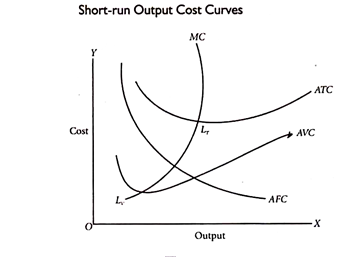
Another important point to be noted is that in Fig. The marginal cost curve (MC curve) intersects both the AVC curve and ATC curve at their minimum points. This is often very simple to explain. If marginal cost (MC) is less than the average cost (AC), it'll pull AC down. If the MC is greater than AC, it'll pull AC up. If the MC is equal to AC, it'll neither pull AC up nor down. Hence, MC curve tends to intersect the AC curve at its lowest point.
Similar is that the position about the average variable cost curve. It’ll not make any difference whether MC goes up or down. LT is the lowest point of total cost and LV is that the lowest point of variable cost.
• If both AFC and AVC fall, ATC will fall.
• If AFC falls but AVC rises
(a) ATC will fall where the drop by AFC is more than the increase in AVC.
(b) ATC won't fall where the drop by AFC is equal to the increase in AVC.
(c) ATC will rise where the drop by AFC is less than the increase in AVC.
Cost Output Relationship in long run
The long run is a period long enough to form all costs variable including such costs as are fixed in the short run. In the short run, variations in output are possible only within the range permitted by the existing fixed plant and equipment. But in the long run, the entrepreneur has before him variety of alternatives which includes the construction of varied kinds and sizes of plants.
Thus, there are no fixed costs since the firm has sufficient time to fully adapt its plant. And all costs become variable. In view of this, the long-run costs will refer to the costs of producing different levels of output by changes within the size of plant or scale of production. The long-run cost-output relationship is shown graphically by the long- run cost curve—a curve showing how costs will change when the scale of production is modified .
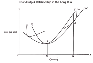
The concept of long-run costs is further explained with the help of an illustration. Suppose that at a specific time, a firm operates under average total cost curve U2 and produces OM. Now it's desired to supply ON. If the firm continues under the old scale, its average cost curve will be NT. If the scale of firm is altered, the new cost curve are going to be U3. The average cost of producing ON will then be NA.
NA is less than NT. Therefore the new scale is preferable to the old one and should be adopted. In the long run, the average cost of producing ON output is NA. This may be called as the long-run cost of producing ON output. It may be noted here that we shall call NA as the long-run cost only so long because the U3 scale is in the planning stage and has not actually been adopted. The moment the scale is installed, the NA cost will be the short-run cost of producing ON output.
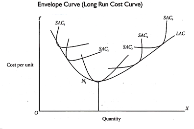
To draw a long-run cost curve, we've to start with a number of short-run average cost curves (SAC curves), each such curve representing a selected scale or size of the plant, including the optimum scale. One can now draw the long-run cost curve which tangential to the entire family of SAC curves, that is, it touches each SAC curve at one point.
In the short run, some inputs are fixed while the others are variable. On the opposite hand, in the long run, the firm can vary all of its inputs. Long run cost is the minimal cost of producing any given level of output when all individual factors are variable. The long run cost curve helps us understand the functional relationship between out and therefore the long run cost of production.
Deriving a long Run average cost Curve
To understand the derivation of a long run average cost curve, let’s consider three short run average cost curves (SACs) as shown in Fig. 1 below.
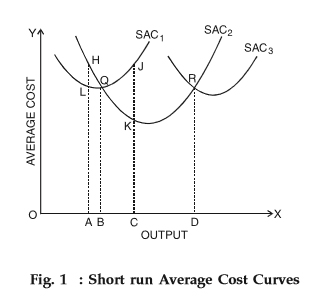
These SACs are called plant curves. In the short run, a firm can operate on any SAC, given the scale of the plant. For the sake of our understanding, let’s assume that there are only three plants that are technically possible. Therefore, the firm increases or decreases its outputs by changing the quantity of the variable inputs.
However, in the long run, the firm examines each SAC to seek out the curve that allows it to produce a given level of output at the minimum cost. Hence, it chooses between SAC1, SAC2, and SAC3. From Fig. 1 above, you'll see that to get OB amount of output, the firm can choose from SAC1 and SAC2. Note that the firm will choose SAC1 because of the lower costs as compared to SAC2.
Further, you'll also see that if the firm tries to produce an output OA, then it costs
• AL per unit with SAC1
• AH per unit with SAC2
Clearly, AH> AL. Therefore, the firm chooses SAC1. Similarly, if the firm tries to produce an output which is greater than OB but OD, then it chooses SAC2 since SAC1 involves higher costs. Also, for outputs larger than OD, the firm uses SAC3. Summing up, we can say that in the long run, the firm employs the plant yielding maximum output at minimum cost per unit.
Imagine if a firm has a choice of varying a plant by infinitely small gradations resulting in infinite average cost curves. In such a case, the smooth curve enveloping of these short-run average cost curves is a long run monetary value curve.
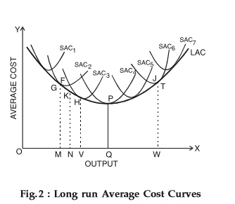
As you'll see in the figure above, the long run average cost curve is drawn tangential to all SACs. In other words, every point on the long run average cost curve is a tangent point on some SAC. Hence, whenever a firm desires to produce a precise output, it operates on the corresponding SAC.
From the Fig. 2 above, you'll observe that to produce an output OM, the corresponding point on the long run average cost curve is ‘G’. Also, the corresponding SAC is SAC2.
Therefore, the firm operates on SAC2 at point G. Similarly, the firm chooses different SACs supported its output requirement. It's also possible for the firm to produce the output OM with SAC3.
However, this will lead to a higher cost of production as compared to SAC2. On the opposite hand, to produce a higher output OV, the firm requires SAC3. If the firm uses SAC2 for the same, then it leads to higher unit similarity.
Note:
The long run average cost curve isn't tangent to the minimum points of the SACs. For that matter, the long run monetary value curve is tangential to
• The falling portions of the SACs while it's declining and
• The rising portions of the SACs while it's rising
Therefore, to produce an output less than OQ at the least cost, the firm operates the plant at less than its full capacity or less than its minimum cost of average production. To create an output larger than OQ at the least cost, the firm operates the plant beyond its optimum capacity.
OQ is that the optimum point because the output OQ is produced at the minimum point of the long run average cost curve and therefore the corresponding SAC (SAC4). While other plants are used at less than or more than their full capacity, only SAC4 is operated at the minimum point.
A long run average cost curve is called as a planning curve. This is often because a firm plans to produce an output within the long run by choosing a plant on the long run average cost curve corresponding to the output. It helps the firm decide the size of the plant for producing the desired output at the least possible cost.
Why does a long run average cost curve have a U-shape?
From Fig. 2, you'll see that the LAC curve (long run average cost curve) is a U-shaped curve. This shape depends on the returns to scale. We know that, as a firm expands, the returns to scale increase.
Then they remain constant for some time and eventually decrease. On the same lines, the LAC curve first declines and eventually rises. Returns to scale have an inverse relationship with the long run average costs. Usually, a firm experiences
• Falling long run average costs and increasing economies to scale because of internal and external economies of scale.
• Rising long run average costs and diminishing economies to scale because of internal and external diseconomies of scale.
Now, the LAC curve shown in Fig. 2 relies on the traditional economic analysis. It's a flattened U-shape which exists only if the state of technology remains constant. However, empirical evidence shows that in the long run, the state of technology changes. Therefore, modern firms face an L-shaped LAC curve as against a U-shaped curve as shown below.
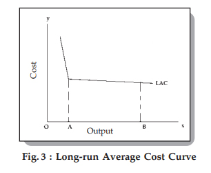
As you'll see above, over the AB range, the curve is perfectly flat. This means that over this range, all sizes of plant have the same minimum cost of production.
The long run refers to that time period for a firm where it can vary all the factors of production. Thus, the long run consists of variable inputs only, and therefore the concept of fixed inputs doesn't arise. The firm can increase the size of the plant in the long run. Thus, you'll well imagine no difference between long-run variable cost and long-run total cost, since fixed costs don't exist within the long run.
Long Run Total Costs
Long run total cost refers to the minimum cost of production. It's the least cost of producing a given level of output. Thus, it can be but or equal to the short run average costs at different levels of output but never greater.
In graphically deriving the LTC curve, the minimum points of the STC curves at different levels of output are joined. The locus of all these points gives us the LTC curve.
Long Run average cost Curve
Long run average cost (LAC) is defined as the average of the LTC curve or the cost per unit of output within the long run. It are often calculated by the division of LTC by the number of output. Graphically, LAC is derived from the Short run average cost (SAC) curves.
While the SAC curves correspond to a particular plant since the plant is fixed within the short-run, the LAC curve depicts the scope for expansion of plant by minimizing cost.
Derivation of the LAC Curve
Note in the figure, that each SAC curve corresponds to a specific plant size. This size is fixed but what can vary is that the variable input within the short-run. In the long run, the firm will select that plant size which might minimize costs for a given level of output.
You can see that till the OM1 level of output it's logical for the firm to operate at the plat size represented by SAC2. If the firm operates at the cost represented by SAC2 when producing an output level OM2, the cost would be more.
So within the long run, the firm will produce till OM1 on SAC2. However, till an output level represented by OM3, the firm can produce at SAC2, after which it's profitable to produce at SAC3 if the firm wishes to minimize costs.
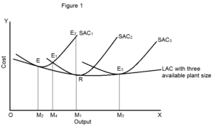
Thus, the choice, in the long run, is to produce at that plant size which will minimize costs. Graphically, this gives us a LAC curve that joins the minimum points of all possible SAC curves, as shown within the figure. Thus, the LAC curve is also called an envelope curve or planning curve. The curve first falls, reaches a minimum then rises, giving it a U-shape.
We can use returns to scale to explain the shape of the LAC curve. Returns to scale depict the change in output with reference to a change in inputs. During Increasing Returns to Scale (IRS), the output doubles by using less than double inputs. As a result, LTC increases less than the rise in output and LAC will fall.
• In Constant Returns to Scale (CRS), the output doubles by doubling the inputs and therefore the LTC increases proportionately with the increase in output. Thus, LAC remains constant.
• In Decreasing Returns to Scale (DRS), the output doubles by using more than double the inputs therefore the LTC increases more than proportionately to the rise in output. Thus, LAC also rises. This gives LAC its U-shape.
Long Run marginal cost
Long run marginal cost is defined at the additional cost of producing an additional unit of the output in the long-run i.e. when all inputs are variable. The LMC curve comes by the points of tangency between LAC and SAC.
Note a very important relation between LMC and SAC here. When LMC lies below LAC, LAC is falling, while when LMC is above LAC, LAC is rising. At the point where LMC = LAC, LAC is constant and minimum.
Learning Curve
The learning curve is a vital modern concept consistent with which cumulative experience in the production of a product over time increases efficiency within the use of inputs like labour and raw materials and thereby lowers cost per unit of output. K.J. Arrow, one among the pioneers in putting forward this idea calls it “Learning by doing”.
According to Arrow, as a firm or its manager produces successive lots of output over various periods of time, it learns to produce more with a given quantity of resources or it's capable of producing a given output by using lesser quantities of inputs or resources than before.
Thus, either with the rise in efficiency of resources or with saving in resources like labour and raw materials, cost per unit of output declines. This learning curve effect mostly occurs in the reduction of labour requirements per unit of output.
A number of factors bring this learning curve effect. As cumulative volume of output over successive periods of time increases, labour and supervisors become more familiar with the work methods or the production process, which results in the reduction within the amount of scrap and other sorts of wastes.
Besides, raw materials cost per unit of output can also decline as cumulative volume of output in successive periods over time increases and as a result a firm gains more experience in doing a production process repeatedly over successive time periods.
The learning curve is graphically shown in Fig. 19.16 where on the X-axis cumulative total output over successive periods of time and on the F-axis cost per unit of output are measured. It’ll be seen from Fig. 19.16 that the learning curve shows downward which shows declining cost per unit of output as cumulative output increases over time and therefore the firm learns from its work experience.
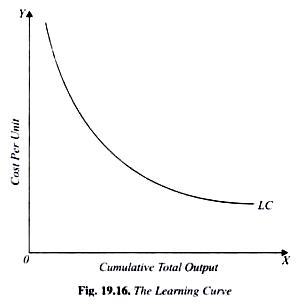
The learning curve effect is usually expressed as a constant percentage. This percentage represents the proportion by which cost per unit of output declines with the increase in cumulative output in each successive time period.
For example, if in a production process labour-input cost experiences 80 per cent learning curve effect, this suggests that if in the first period production of a unit of output requires labour cost of Rs. 1000, in the next period labour cost per unit will decline to Rs. 800 then forth.
Meaning of Break-Even Point:
Break-even point represents that volume of production where total costs equal to total sales revenue resulting into a no-profit no-loss situation.
If output of any product falls below that point there's loss; and if output exceeds that point there's profit.
Thus, it's the minimum point of production where total costs are recovered therefore, at break-even point.
Sales Revenue – Total Cost
Or, Sales – Variable Cost = Contribution = fixed cost
It is concluded that at break-even point the contribution earned just covers the fixed charge and, at levels below the point, contribution earned isn't sufficient to match the fixed cost and, at levels above the point, contribution earned more than recovers the fixed cost.
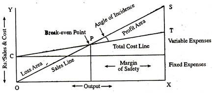
P is the break-even point in the break-even chart where OS and CT—being the sales line and total cost line—intersects. A loss result in the left side of P, i.e., before the break-even point is reached, and, beyond P, profit starts to generate. Break-even point has a wide use within the field of marginal costing and helps to decide the product mix, fixation of selling price, steps to be taken in long-term planning etc.
Break-even point is ascertained by using the subsequent formula:

Assumptions Underlying Break-Even Analysis:
The break-even analysis relies on certain assumptions.
They are:
(i) All costs is separated into fixed and variable components,
(ii) Fixed costs will remain constant at all volumes of output,
(iii) Variable costs will fluctuate in direct proportion to volume of output,
(iv) Selling price will remain constant,
(v) Product-mix will remain unchanged,
(vi) The number of units of sales will coincide with the units produced so that there's no opening or closing stock,
(vii) Productivity per worker will remain unchanged,
(viii) There'll be no change in the general price level.
Uses of Break-Even Analysis:
(i) It helps within the determination of selling price which can give the desired profits.
(ii) It helps within the fixation of sales volume to cover a given return on capital employed.
(iii) It helps in forecasting costs and profit as a results of change in volume.
(iv) It gives suggestions for shift in sales mix.
(v) It helps in making inter-firm comparison of profitability.
(vi) It helps in determination of costs and revenue at various levels of output.
(vii) It’s an aid in management decision-making (e.g., make or buy, introducing a product etc.), forecasting, long-term planning and maintaining profitability.
(viii) It reveals business strength and profit earning capacity of a concern without much difficulty and energy.
Limitations of Break-Even Analysis:
1. Break-even analysis relies on the assumption that all costs and expenses is clearly separated into fixed and variable components. In practice, however, it may not be possible to attain a clear-cut division of costs into fixed and variable types.
2. It assumes that fixed costs remain constant at all levels of activity. It should be noted that fixed costs tend to vary beyond a particular level of activity.
3. It assumes that variable costs vary proportionately with the quantity of output. In practice, they move, no doubt, in sympathy with volume of output, but not necessarily in direct proportions..
4. The assumption that selling price remains unchanged gives a straight revenue line which cannot be true. Selling price of a product depends upon certain factors like market demand and supply, competition etc., so it, too, hardly remains constant.
5. The assumption that just one product is produced or that product mix will remain unchanged is difficult to seek out in practice.
6. Apportionment of fixed cost over a range of products poses a problem.
7. It assumes that the business conditions might not change which isn't true.
8. It assumes that production and sales quantities are equal and there'll be no change in opening and closing stock of finished product, these don't hold good in practice.
9. The break-even analysis doesn't take into consideration the amount of capital employed in the business. In fact, capital employed is a vital determinant of the profitability of a concern.
The formula for calculating the break-even point is
ВЕР– Total Fixed Cost/Contribution Margin Per Unit
Contribution margin per unit can be obtained by by deducting the average variable cost from the selling price. Therefore the formula is
BEP = Total Fixed Cost/Selling Pr ice – AVC
Example:
Suppose the fixed cost of a factory in Rs. 10,000, the selling price is Rs. 4 and therefore the average variable cost is Rs. 2, therefore the break-even point would be
ВЕР = 10,000(4-2) = 5,000 units.
It means if the corporate makes the sales of 5,000 units, it might make neither loss nor profit. This will be seen in the analysis.
Sales = Rs.20, 000
Cost of products sold:
(a) Variable cost at Rs.2 = Rs. 10,000
(b) Fixed costs = Rs. 10,000
Total Cost = Rs. 20,000
Net Profit = Nil
ВЕР in term of Sales Value:
Multi-product firms aren't in a position to measure the break-even point in terms of any common unit of product. They find it convenient to determine the break-even point in terms of total rupee sales. Here again the break-even point would be where the contribution margin (sales value—variable costs) would be adequate to fixed costs. The contribution margin however, is expressed as a ratio to sales. The formula for calculating the break-even point is
BEP = Fixed Cost/Contribution Ratio
Contribution Ratio (CR) = Total Revenue (TR)-Total Variable Cost (TVC)/Total Revenue (TR)
For example, if TR is Rs. 600 and TVC is Rs. 450, then the contribution ratio is
CR = 600 – 450/600/600=150/ 600 = 0.25
The Contribution Ratio is 0.25
BEP = Total fixed cost /Contribution Ratio
= 150/0.25 = 600
The firm achieves its ВЕР when its sales are Rs. 600
Total Revenue = Rs.600
Total Cost = Rs.600
Net Profit/loss = Nil
Types of Break-Even Point:
The above paragraph explains an easy sort of break-even point which is based on cost and revenue i.e., the profit and loss break-even.
There are two other sorts of break-even and that they are:
(i) Cash break-even, and
(ii) Income break-even.
(i) The Cash Break-Even:
An industry requires money for 2 purposes i.e., to acquire capital assets and to satisfy working capital requirements. These requirements are often partly met by his own investment and partly by loans and advances from financial institutions. The industry requires term loans to acquire capital assets like land and building, plant and machinery.
In the case of term loans, the financial institutions shall have to determine the probability of the applicant being able to satisfy the interest and loan repayment schedule. It'll be more interested in knowing the level of break-even point where not only total costs are required but also the full debt service.
The level of break-even is named the cash break-even. It's based on revenue and cost data involving cash flows. The depreciation, investment allowance reserve and other provision of the cost items should be excluded but at an equivalent time the repayment of installment should be added to fixed cost.
Cash Break-Even Point = Fixed Cost+ Loan installment – Cash outflow/Contribution per unit
(ii) The Income Break-Even:
The various sources from which the industry is proposed to be financed like the capital, long term borrowing, deferred payments and other sources. If these sources are inadequate the industry may approach the bank for under writing its shares. If the share market doesn't respond positively, the equity risk falls on the underwriter.
As the shareholder of the bank will expect a certain dividend just to cover the payment of interest for the term loans so as to calculate income break-even point the equity capital cash earnings should be added. The income breakeven point is calculated in the following manner.
Income Break-Even Point = fixed cost + Earnings required for dividend/Contribution per unit
Multiple-product Firms and Break-Even Point:
The multiple products may differ in models, styles or sizes of their output. Within the case of multiproduct firms the break-even point for every product are often calculated if the ‘product mix’ is understood. The product mix is the full list of products offered for sale by a corporation. It may range from one or two product lines to a combination of several product lines or groups.
Suppose an industry is engaged within the production of three items, namely X, Y, and Z. The contribution for items is as follows:
X = Rs. 6 per unit
Y = Rs. 4 per unit
Z = Rs. 2 per unit
The product-mix given by the manufacturer is as follows:
X = 40,000 units
Y = 2, 00,000 units
Z = 1, 60,000 units.
Then the product-mix proportions are 1:5:4. We will compute the weighted average contribution within the following way:
Product – Contribution x Unit Proportions – Total Contributions
X – 6 x 1 – 6
Y – 4 x 5 – 20
Z – 2 x 4 – 8
Your time
10 – 34
Average Contribution per unit = 34/ 10 = Rs 3.4
BEP= Total Fixed Cost/ Average contribution per unit = 5, 10,000 / 3.4 = 1, 50,000 units
We will get the break-even output for all the three items by dividing the above figure within the same proportion
X = 15,000
Y = 75,000
Z = 60,000
This reveals that the production manager has got to ensure that production in the X line doesn't go below 15,000 units, in the Y line 75,000 units and within the Z line 60,000 units. If not, he has got to sustain loss. The same method is applied for computing the ВЕР in cases of multiple product industries produc¬ing any number of items.
The break-even analysis is used for the subsequent purposes:
(i) Safety Margin:
The break-even chart helps the management to understand at a glance the profits generated at the varied levels of sales. The safety margin refers to the extent to which the firm can afford a decline before it starts incurring losses.
The formula to work out the sales margin of safety is:
Safety Margin= (Sales – BEP)/ Sales x 100
From the numerical example at the extent of 250 units of output and sales, the firm is earning profit, the safety margin are often found out by applying the formula
Safety Margin = 250- 150 / 250 x 100 =40%
This means that the firm which is now selling 250 units of the product can afford to decline sales up to 40 per cent. The margin of safety could also be negative also , if the firm is incurring any loss. Therein case, the percentage tells the extent of sales that ought to be increased so as to reach the point where there'll be no loss.
(ii) Target Profit:
The break-even analysis can be utilised for the aim of calculating the volume of sales necessary to realize a target profit.
When a firm has some target profit, this analysis will help find out the extent of increase in sales by using the subsequent formula:
Target Sales Volume = fixed cost + Target Profit / Contribution Margin per unit
By way of illustration, we can take Table 1 given above. Suppose the firm fixes the profit as Rs. 100, then the volume of output and sales should be 250 units. Only at this level, it gets a profit of Rs. 100. By using the formula, an equivalent result will be obtained.
(iii) Change in Price:
The management is often faced with a problem of whether to reduce prices or not. Before taking a decision on this question, the management will need to consider a profit. a reduction in price leads to a reduction in the contribution margin.
This means that the quantity of sales will need to be increased even to keep up the previous level of profit. The higher the reduction in the contribution margin, the higher is that the increase in sales needed to ensure the previous profit.
The formula for determining the new volume of sales to maintain the same profit, given a reduction in price, is going to be as follows:
New Sales Volume = Total fixed cost = Total Profit/ New selling price – Average Variable Cost
For example, suppose a firm has a fixed cost of Rs. 8,000 and therefore the profit target is Rs.20, 000. If the sales price is Rs.8 and therefore the average variable cost is Rs. 4, then the total volume of sales should be 7,000 units on the basis of the formula given under target price.
Suppose the firm decides to reduce the selling price from Rs.8 to Rs. 7, then the new sales volume should be on the basis of the above formula:
New Sales Volume = 8,000 + 20,000/7-4 = 9,300
From this, we will infer that by reducing the price from Rs. 8 to Rs. 7, the firm has got to increase the sales from Rs. 7,000 to Rs 9,330 if it wants to keep up the target profit of Rs. 20,000. Within the same way, the sales executive can calculate the new volume of sales if it increases the price.
(iv) Change in Costs:
When costs undergo change, the selling price and therefore the quantity produced and sold also undergo changes.
Changes in cost can be in two ways:
(i) Change in variable cost, and
(ii) Change in fixed cost.
(i) Variable Cost Change:
An increase in variable costs results in a reduction in the contribution margin. This reduction in the contribution margin will shift the break-even point downward. Conversely, with the fall within the proportion of variable costs, contribution margins increase and break-even point moves upwards.
Under conditions of changing variable costs, the formula to determine the new quantity or the new selling price is:
(a) New Quantity or Sales Volume = Contribution to Margin/ Present selling price – New Variable Cost per Unit
(b) New selling price = Present Sale Price +New Variable Cost-Present Variable Cost
Example:
The contribution margin is Rs. 64,000, this sale price is Rs.10 and therefore the present variable cost is Rs.6. If the variable cost per unit goes up from Rs.6 to Rs. 7, what will be the new sales volume and price?
New Sales Volume = 64,000/ 10-7 = 64,000 /3 = 21,300 units
New Sales Price = (106) = Rs. 11.
(ii) Fixed cost Change:
An increase in fixed charge of a firm is also caused either because of a tax on assets or because of a rise in remuneration of management, etc. it'll increase the contribution margin and thus push the break-even point upwards. Again to maintain the earlier level of profits, a new level of sales volume or new price has to be found out.
New Sales Volume = Present Sale Volume +
(New fixed cost + Present Fixed Costs)/ (Present Selling Price-Present Variable Cost)
New Sale Price = Present Sale Price +
(New Fixed Costs – Present Fixed Costs)/ Present Sale Volume
Example:
The fixed cost of a firm increases from Rs. 5,000 to Rs. 6,000. The variable cost is Rs. 5 and therefore the sale price is Rs. 10 and therefore the firm sells 1,000 units of the product
New Sales Volume = 1,000 + 6,000 – 5,000/ 10 – 5 =1,000 + 1,000/ 5 = 1,000 + 200=1,200 units
New Sale Price = 10 + 6,000 – 5,000/ 1,000 = 10 + 1,000/ 1,000= Rs.10 + Re1
= Rs. 11
(v) Decision on Choice of Technique of Production:
A firm has to decide about the most economical production process both at the planning and expansion stages. There are many techniques available to produce a product. These techniques will differ in terms of capacity and costs. The break¬even analysis is that the most simple and helpful within the case of decision on a choice of technique of production.
For example, for low levels of output, some conventional methods is also most probable as they require minimum fixed cost. For high levels of output, only automatic machines is also most profitable. By showing the cost of different alternative techniques at different levels of output, the break-even analysis helps the selection of the choice among these techniques.
(vi) Make or Buy Decision:
Firms often have the option of making certain components or for purchasing them from outside the concern. Break-even analysis can enable the firm to choose whether to make or buy.
Example:
A manufacturer of car buys a particular components at Rs. 20 each. Just in case he makes it himself, his fixed and variable cost would be Rs. 24,000 and Rs.8 per component respectively.
BEP = Fixed Cost/ purchase price – Variable Cost
= 24,000/ 20-8 = 24,000/ 12 = 2,000 units
From this, we will infer that the manufacturer can produce the parts himself if he needs more than 2,000 units per annum . However, certain considerations got to be taken account of in a buying decision, such as
(i) Is that the required quality of the product available?
(ii) Is that the supply from the market certain and timely?
(iii) Do the supplies of the components try to take any monopoly advantage?
(vii) Plant Expansion Decisions:
The break-even analysis is also adopted to reveal the effect of an actual or proposed change in operation condition. This might be illustrated by showing the impact of a proposed plant on expansion on costs, volume and profits. Through the break-even analysis, it might be possible to examine the varied implications of this proposal.
Example:
A company has the capacity to produce goods worth of Rs. 40 crores a year. For this has incurred a fixed cost of Rs 20 crores, the variable costs being 60% of the sales revenue. Now company is planning to incur an extra Rs. 6 crores in feed costs to expand its production capacity from Rs. 40 crores to Rs.60 crores. The survey shows that the firm’s sales are increased from Rs. 40 crores to Rs. 50 crores. Should the firm get in for expansion?
ВЕР at the present capacity = Fixed cost/ Margin Contribution% = Rs. 10 crores/ 40% =Rs25Crores
ВЕР at the proposed capacity = Rs 16 crores/40%= Rs 40 crores.
Increase in break-even point = Rs 40 crores-Rs. 25 crores = Rs. 15 crores.
Thus we can infer that the firm should get in for expansion as long as its sales expand by more than Rs. 15 crores from its earlier level of Rs. 40 crores.
(viii) Plant shut down Decisions:
In the pack up decisions, a distinction should be made between out of pocket and sunk costs. Out of pocket costs include all the variable costs plus the fixe cost which don't vary with output. Sunk fixed costs are the expenditures previously made but from which benefits still remain to be obtained e.g. Depreciation.
(ix) Advertising and Promotion Mix Decisions:
The main objective of advertisement is to stimulate or increase sales to all customers-former, present and future if there's keen to undertake vigorous campaign of advertisement. The management has got to examine those marketing activities that stimulate consumer purchasing and dealer effectiveness.
The break-even point concept helps the management to understand about the circumstances. It enables him not only to take appropriate decision but by showing how these additional fixed charge would influence BEPs. The advertisement pushes up the total cost curve by the amount of advertisement expenditure.
Limitations:
We may now mention some important limitations which need to be kept in mind while using break-even analysis:
1. In the break-even analysis, we keep everything constant. The selling price is assumed to be constant and therefore the cost function is linear. In practice, it'll not be so.
2. In the break-even analysis since we keep the function constant, we project the future with the help of past functions. This is often not correct.
3. The belief that the cost-revenue-output relationship is linear is true only over a small range of output. It's not an effective tool for long-range use.
4. Profits are a function of not only output, but also of other factors like technological change, improvement in the art of management, etc., which are overlooked in this analysis.
5. When break-even analysis is based on accounting data, because it usually happens, it may suffer from various limitations of such data as neglect of imputed costs, arbitrary depreciation estimates and inappropriate allocation of overheads. It are often sound and useful only if the firm in question maintains a good accounting system.
6. Selling costs are especially difficult to handle break-even analysis. This is often because changes in selling costs are a cause and not a results of changes in output and sales.
7. The simple sort of a break-even chart makes no provisions for taxes, particularly corporate income tax.
8. It usually assumes that the price of the output is given. In other words, it assumes a horizontal demand curve that's realistic under the conditions of perfect competition.
9. Matching cost with output imposes another limitation on break-even analysis. Cost in a particular period needn't be the results of the output in that period.
10. Because of numerous restrictive assumptions underlying the technique, computation of a breakeven point is considered an approximation instead of a reality.