UNIT IV
Standard Costing and Variance Analysis
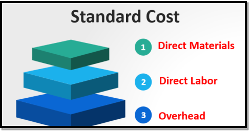
Standard Costing
It is a standard or a benchmark. It is useful for comparison. It may show minimal quality. For eg. - Standard of passing.
Standard cost
Under normal conditions, the standard cost estimated or pre-determined cost of performing an operation or producing a good or service. It is used as the basis for cost control with variance analysis. It is selected to serve as a benchmark for Standard Costing/Budget Control Systems. This is the budget for the production of one unit of a product or service. It is a cost that is calculated from the management's effective operation and relevant necessary expenditure standards.
Standard costing
This is a cost accounting technique for cost control, in which standard costs are determined, compared with actual costs, and corrective actions are initiated.
This is a method of control, which involves the creation of detailed costs and sales budgets. A management tool used to facilitate management by exceptions.
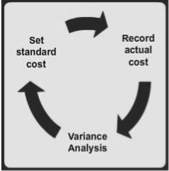
Set a standard cost
The standard quantity is predetermined and the standard price per unit is estimated. Budget costs are calculated using standard costs.
Record the actual cost
Calculate the actual quantity and the cost incurred to give the full details.
Analysis of variance
Compare actual and budget costs. Cost variances are used in cost control. Take appropriate corrective action.
Fixed liability compliance (legal compliance) is an effective control system. If necessary, reset the budget.
Types of standards ideal standards:
These are used when the price for materials and labor is most favorable, when the highest output is achieved with the best equipment and layout and when the minimum cost are low.
- Normal standard:
. Normal activity is defined as the number of Standard Times in which a normal efficiency produces enough goods to meet the average annual sales demand.
2. Basic or bogey standards:
These criteria are used only if they can remain constant or unchanged for a long time. According to this criterion, the base year is selected for comparative purposes in the same way that statisticians use price indices.
If the basic standard is used, the variance is not calculated as the difference between the standard and actual costs. Instead, the actual cost is represented as a percentage of the base cost.
3. Current standards:
These criteria reflect management's expectations for the actual costs of the current period. These are the costs incurred by the business owner if the expected price is paid for the goods and services and the use corresponds to what is deemed necessary to generate the planned output.
Dispersion
The difference between the standard cost and the actual cost of the actual output is defined as a variance. Dispersion may be beneficial or unfavorable.
If the actual cost is less than the standard cost, the variance is advantageous; if the actual cost is greater than the standard cost, the variance is unfavorable.
In practice, it is not enough to know the numbers of these differences, and to take the necessary corrective actions to reduce/eliminate them, it is necessary to track their origin and cause of occurrence.
Distributed type
The purpose of the quality costing report is to research the explanations for significant differences so as to spot problems and take corrective action. Dispersion is largely two types, namely, controllable and uncontrollable.
Controllable dispersion
A controllable variance is a variance that can be controlled by the department head, while an uncontrollable variance is a variance that exceeds their control. If the unruly differences are of a material nature and are permanent, then the Standard may require revision.
Analysis of variance
Anova is to divide the cost variance into its components and know what is causing it.
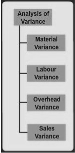
Take corrective action for the approach.
Efficiency dispersion: Variations that arise due to the amount of material, the effectiveness in the use of Labor. Here we compare the actual quantity with the given criteria.
Price rate differences: Differences resulting from changes in unit material prices, Standard Working Hours rates, and standard allowances for overhead costs. Here the actual price is compared with the prescribed one.
Difference by volume: Variance due to the effect of the difference between the actual activity and the level of activity estimated when the criterion was set.
Reasons for material dispersion
- Change of base price.
- The expected standard quantity cannot be purchased at the appropriate price. Use of sub-standard materials.
- Ineffective use of materials. Pilferage
- Material difference Material cost variance=(standard quantity X standard price)-(actual quantity X method price) Item price difference=actual quantity(standard price-actual price)
- Material usage variance=standard price(standard quantity-actual quantity)
- The reasons for problems related to Labor variance time.
- Changes in design and quality standards. Low motivation.
- Poor working conditions.
- Improper scheduling/labor placement. Insufficient training.
- Rate-related issues. Increment/high labor wage. Overtime.
- Labor shortages lead to higher rates. Union contract.
- Labor dispersion Labor cost variance=(standard time X Standard Time)–(actual hours X actual hours)
- Labor rate variation = actual time (standard rate-actual rate)
- Labor efficiency variance=standard rate (Std Hrs-actual Hrs worked)
- Idle time variance=idle time X Std rate
Reasons for overhead distribution
- Absorption under or above fixed overhead. Reduced demand/improper planning.
- Failure/power failure. Labor issues.
- Inflation
- Lack of planning.
- Lack of cost control.
Variable overhead (Oh) variance
Variable OH cost variance= (standard time X standard variable Oh rate)–actual Oh cost
Variance of variables in Ohio
Variable OH expenditure variance = (actual time × standard variable Oh rate)–actual OH cost
Variable OH efficiency variance = (standard Hrs-actual hrs) X standard variable Oh rate
Fixed overhead (Oh) dispersion
Fixed OH cost variance=absorption Oh-actual Oh absorption Oh=actual unit*standard OH rate per unit
We fixed the oh dispersion.
Fixed Oh expenditure variance=budget Oh-actual Oh fixed Oh volume variance=absorption Oh-budget Oh
Reasons for sales fluctuations
- Price changes. Changing market size.
- Change in market share.
- Sales variance
- Sales difference=budget sales-actual sales
- Sales price variance=actual quantity(actual price-budget price)
- Sales quantity variance=budget price(actual quantity-budget quantity)
Advantages of Standard Costing
- Basis for sensible cost comparison.
- Employment of management by exception. Means of performance evaluation for employees. Product cost results more stable.
Disadvantages of Standard Costing
- This is a great app as it takes time because it's too comprehensive. Accurate estimation of prices and rates is difficult.
- Requires continuous revision with frequent changes in technology/market trends. Focus on minimizing costs, not quality or innovation.
- Material difference
- Material cost variance material price difference material use variance
Can i sub-split the usage variance?
When we have multiple raw materials, what is the cause?
Material difference
Material cost variance material price difference material use variance material yield variance material mixture variance
Material cost variance=(standard quantity X standard price) - (actual quantity X Act Price)material price variance=actual quantity (standard price-actual price)
Material use variance=standard price(standard quantity-actual quantity)material yield variance=(Std input quantity-actual input Qty)*Std price of Std input material mixture variance = standard price(revised standard quantity-actual quantity))
Fixed overhead (Oh) dispersion
Fixed OH cost variance=absorption Oh-actual Oh absorption Oh=actual unit*standard OH rate per unit
We fixed the oh dispersion.
Fixed Oh expenditure variance=budget Oh-actual Oh fixed Oh volume variance=absorption Oh-budget Oh
Material difference
F OH cost difference
F Oh expenditure variance F Oh volume variance
Can i sub-split the volume variance?
What is its cause and why does the volume change?
We fixed the oh dispersion.
Fixed OH efficiency variance=standard Oh rate/time(standard Hrs-actual hrs)fixed Oh capacity variance = standard Oh rate / time (budget hours actual hours actual hours actual hours actual hours actual hours actual hours actual hours actual hours actual hours actual hours actual hours


Standard costing is an important management tool, so you need to provide important information during installation. The following steps are required to establish a standard costing system in your organization:
1. Determining the cost center
Cost centers are needed to fix costs and responsibilities. For manufacturing, a cost center is created according to the number of products produced, which determines the number of sections, departments, or departments involved in the production process. Cost centers related to people are called personnel cost centers, and cost centers related to products and equipment are called non-personal cost centers.
2. Account classification
Costs are incurred at various stages of the manufacturing process. These costs should be properly recorded in order to accurately calculate the total costs incurred. Therefore, you need to classify your accounts for cost control under the standard costing system.
3. Account coding
You can organize different accounts and use different symbols to facilitate quick collection, communication, and reporting. The following code can be used for the cost factor.
4. Criteria setting
Criteria are ideally expected and can be achieved in future periods, usually in the next fiscal year. The success of standard costing systems is based on the authenticity, reliability, and acceptance of these standards.
There are three types of standards. They are the current standard, the basic standard, and the regular standard. The current standard is divided into two, the ideal standard and the expected or achievable standard.
5. Establishment of standard cost
Standard costs are set individually for each cost element. In general, cost elements are grouped as materials, labor, and overhead costs. In addition, standard costs are set for sales.
6. Preparation of standard cost card or standard cost sheet
Standard cost cards or standard cost sheets are created separately for each product or process.
7. Standard costing organization
A committee is formed to set the standards. If so, the purpose of the standard costing system can be easily achieved.
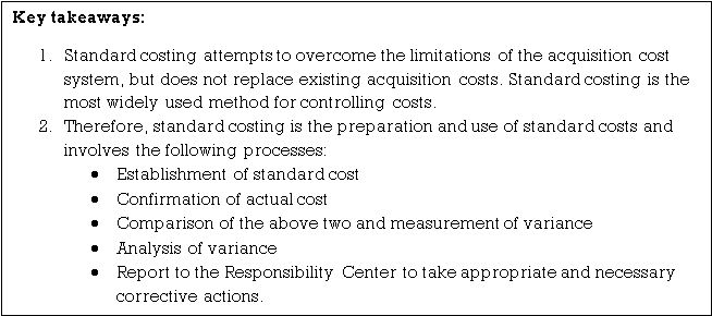
The standard function in costing is to reveal the variance between the allowed standard cost and the recorded actual cost. The Chartered Institute of Management Accountants (UK) defines variance as the difference between standard cost and equivalent actual costs incurred during the period. Variance analysis can be defined as the process of calculating the amount of variance between the actual cost and the standard cost and identifying its cause. ANOVA has two phases.
(1) Calculation of individual differences and
(2) Identification of the cause of each difference.
I. Material differences:
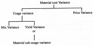
The following variances make up the material variances:
Material cost variance:
Material cost variance is the difference between the actual cost of the direct material used and the standard cost of the direct material specified for the output achieved. This difference is due to the difference between the amount consumed and the amount of material allowed to be produced, and the difference between the price paid and the pre-determined price.
This can be calculated using the following formula:
Material cost variance = (AQ X AP) – (SQ X SP)
Where AQ = Actual quantity
AP = Actual price
SQ = Standard quantity for the actual output
SP = Standard price
Differences in material usage:
Differences in the amount or amount of material used occur when the actual amount of raw material used for production differs from the standard amount that should have been used to produce the achieved output. It is that part of the direct material cost variance that results from the difference between the quantity actually used and the standard quantity specified.
As an expression, this variance is shown as:
Calculate the difference in material usage from the following information:
Standard material cost per unit Issued material
Material A-2 pcs @Rs. 10 = 20 (Material A 2,050 pieces)
Material B-3 pieces @Rs. 20 = 60 (Material B 2,980 pieces)
Total = 80
Completed units 1,000
Solution:
Material usage variance = (Actual Quantity – Standard Quantity) x Standard Price
Material A = (2,050 – 2,000) x Rs. 10 = Rs. 500 (unfavorable)
Material B = (2980 – 3000) x Rs. 20 = Rs. 400 (favorable)
Total = Rs. 100 (unfavorable)
Note that the standard is used to calculate the usage variance, not the actual price. Using the actual price introduces a price factor into the quantity variance. These two elements should be kept separate as different departments are responsible
a) Material mixing variances: Material variances or quantity variances can be divided into mixing variances and yield variances.
For certain product and processing operations, material mixing is an important instrumental variable, and certain grades of material and quantity are determined prior to production. Mixing differences occur if the ingredients are not actually produced in the same proportions as the standard formulation.
For example, if you add 100 kg of raw material A and 200 kg of raw material B to make a product, the standard material mix ratio is 1: 2.
The raw materials actually used must have this 1: 2 ratio. If not, you will find differences in the mix of materials. Differences in material mix are commonly found in industries such as textiles, rubber and chemicals. Mixing differences can occur when cost savings, effective resource utilization, and the amount of raw materials required are not available at the required time. ..
Material mixing differences are part of the material quantity differences due to differences between the actual composition of the mixture and the standard mixture.
It can be calculated using the following formula.
Material mixing variance = (standard price of actual quantity of actual mixture – standard price of actual quantity of standard mixture)
The revised standard mix or ratio is calculated as follows:
Standard mixture of specific materials / standard total amount x actual input
Example:
The product is made from two raw materials, Material A and Material B. One unit of finished product requires 10 kg of material.
Calculate the variance of the material mixture.
Material A- 20% - 2kg @ Rs 20 = Rs 40
 Material B- 80% - 8kg @ Rs 10 = Rs 80
100% - 10 kg@ Rs 12 = Rs 120
Revised standard proportion=
 Standard proportion of a particular mix ×Actual input
Total standard quantity
Revised standard proportion:
Material A = 2/10 × 12 = 2.40 kg.
Material B = 8/10 × 12 = 9.60 kg.
Material mix variance:
Material A= (8 kg – 2.40 kg) × 20
= 5.60 × 20 = 112.0 (unfavorable)
Material B= (4 kg – 9.60) ×1.00
= 5.60 × 10 = Rs 56 (favorable)
Total mix variance= Rs 56 (unfavorable)
b) Difference in material yield:
Material yield variances account for the rest of the total material variances. The difference between the actual yield obtained and the specified standard yield (in terms of actual input) is due to the difference in material usage. In other words, a yield difference occurs when the output of the final product does not match the output obtained using the actual inputs. In some industries, such as sugar, chemicals, and steel, actual yields may differ from expected yields based on actual inputs, resulting in variable yields.
The sum of the material mix variance and the material yield variance is equal to the material quantity or usage variance. If there is no material mixture variance, the material yield variance is equal to the total material quantity variance. Therefore, the difference between mixing and yield is additive, explaining the different parts of the difference in total material usage.
The formula for calculating the yield variance is:
Yield Variance = (Actual yield – Standard Yield specified) x Standard cost per unit
Example:
Standard input = 100 kg, standard yield = 90 kg, standard cost per kg output = Rs 200
The actual input is 200 kg and the actual yield is 182 kg. Calculate the yield variance.
Solution:
Standard yield for the actual point = 90/100 × 200 = 180 kg
 Yield variance = (Actual yield – Standard yield for the actual input) × Standard cost
= 182- 180× Rs 200
= 2 × 200 = Rs 400 (favorable)
The above yield variance can be computed by using another formula also, e.g.,
 Yield Variance = (Actual Loss – Standard Loss on Actual Input) × Standard Cost per
= (18 kg -20 kg) × Rs 200
= Rs 400 (favorable)
In this example, the material usage variance is equal to the material yield variance because there is no mixing variance.
The above formula uses output or loss as the basis for calculating the yield variance. Yield variance can also be calculated based solely on the input coefficients. The fact is that the loss of input is equal to the loss of output. Low yield simply means that a large number of inputs are being used and the expected or standard output (based on the actual inputs) has not been achieved.
Yields in such cases are called sub-usage variances (or revised usage variances) and can be calculated using the following formula:
Sub-usage or revised usage variance = (Revised Standard Proportion of Actual Input – Standard quantity) x Standard Cost per unit of input
Example:
Below are the standard materials and standard prices for manufacturing a unit of product.
Standard material Standard price
Material A 5 kg @ Rs 40
Material B 3 kg @ Rs 60
The actual production of the product is 400 units.
The actual material A 2,500 kg @ Rs 39
B 1,000 kg @ Rs 62.5
Calculate the material sub-usage variance.
Solution:
Revised standard proportion of catual input:
Material A = 5/8 × 3,500 = 2,187.5 kg
Material b = 3/8 × 3,500 = 1,312.5 kg
Material sub-usage variance:
(Revised standard proportion of actual input-Standard quantity) × SP
Material A = (2,187.5 – 2,000) × 40
= 187.5 × 40 = Rs 7,500 (unfavorable)
Material B = (1,312.5 – 1,200) × 60
= 112.5 × 60 = Rs 6,750 (unfavorable)
Total material sub-usage variance = Rs 14,250 (unfavorable)
Or
(3,500 – 3,200) × RS 1,52,000/3,200
= 300 ×1,52,000 /3,200 = Rs 14,250 ( unfavorable)
Differences in material yield are always equal to differences in sub-use. The only difference is in the calculation. The former considers the output or output loss, and the latter considers the standard input and the actual input used for the actual output. Both mixing and yield fluctuations provide useful information for production control, performance assessment, and operational efficiency reviews.
Item price difference:
If the raw material is purchased at a price different from the standard price, there will be a difference in the material price. It is that part of the material directly that results from the difference between the actual price paid and the specified standard price, and the cost difference multiplied by the actual quantity. Expressed as an expression
Differences in material prices are not desirable if the actual price paid exceeds the prescribed standard price. It is recommended that material price variances be calculated for purchased materials, not for used materials. Purchasing materials is an earlier event than using materials.
Therefore, variances based on purchase quantity are basically faster reports than variances based on actual quantity used. This is very beneficial in terms of performance measurement and corrective action. Early reports can help administrators measure performance, correct performance degradation, and scale performance gains early.
By recognizing fluctuations in material prices at the time of purchase, companies can carry all units of the same material at one price (standard cost of material) without having to purchase all units of the same material at the same price. I can do it. Using one price for the same material equipment management simplifies accounting work.
If no direct material price variance is recorded until the material is issued for production, the direct material will be booked at the actual purchase price. Deviations from the standard price of the actual purchase price may not be known until the material is directly issued for production.
Example:
In Example 1, if material A was purchased at a rate of Rs 10 and material B was purchased at a rate of Rs 21, the price variances for the materials would be:
Materials price variance = (Actual Price – Standard Price) x Actual Quantity
Material A = (10 – 10) x 2,050 = Zero
Material B = (21 – 20) x 2,980 = 2980 (un-favorable)
Total material price variance = Rs 2980 (un-favorable)
The total of materials usage variance and price variance is equal to materials cost variance.
II. Labor differences:
If the actual labor cost differs from the standard labor cost, there will be a direct labor cost difference. The labor cost analysis focuses on labor rates and working hours.
Labor differences make up:

Labor cost variance: The labor cost variance indicates the difference between the actual direct wage paid and the standard direct wage specified for the results achieved.
This difference is calculated using the following formula:
Labor cost variance = (AH x AR) – (SH x SR)
Where:
AH = Actual hours
AR = Actual rate
SH = Standard hours
SR = Standard rate
- Difference in labor efficiency:
The calculation of labor efficiency or usage variance follows the same pattern as the calculation of material usage variance. Labor efficiency differences occur when labor operations are more efficient or less efficient than standard performance. Differences in labor efficiency occur when the actual direct working hours required to complete a job differ from the specified standard hours. This is the difference between the actual hours spent and the specified standard hours worked, multiplied by the standard hours worked per hour.
The difference in labor efficiency is calculated by applying the following formula.
Labor efficiency variance = (Actual hours – Standard hours for the actual output) x Std. Rate per hour.
(I) Dispersion of labor mix:
Labor mixed dispersion is calculated in the same way as material mixed dispersion. Manufacture or completion of work requires workers of different types or grades, and if the workers are mixed according to standard proportions, production is complete. In some situations, the standard workforce may not be adhered to and alternatives may need to be made. There may be changes in the wage rates of some workers. You may need to use a more skilled or expensive type of workforce, such as hiring men instead of women. Sometimes workers and operators are absent.
These lead to the emergence of labor composition variances calculated using the following formula:
Labor composition variance = (actual labor composition – revised standard labor composition for actual total hours) x standard rate per hour
For example, the standard labor cost data per factory unit is as follows:
Class | Proportion |
|
|
|
A | 50% | 3 hours @ | Rs 40 | = Rs120 |
B | 50% | 3 hours @ | Rs 20 | = Rs 60 |
| 100% | 6 hours | Rs 30 | Rs 180 |
At one point, many Class B workers were absent and had to be replaced by Class B workers. Class A workers had less work experience, so more working hours were used.
The recorded costs of the unit are:
Class | Proportion |
|
|
|
A | 75% | 6 hours @ | Rs 40 | = Rs240 |
B | 25% | 2 hours @ | Rs 20 | = Rs 40 |
| 100% | 6 hours | Rs 30 | Rs 280 |
The variance of the labor composition is calculated as follows.
Labor composition variance = (actual ratio – revised standard ratio of actual total hours) x standard rate per hour
Revised standard ratio:
Class A = 3/6 × 8 = 4 hours
Class B = 3/6 × 8 = 4 hours
Applying the formula:
Class A = (6-4) × Rs 40 = 80(unfavorable)
Class B = (2-4) × Rs 20 = Rs 40 (favorable)
Total labor mix variance = Rs 40 (unfavorable)
(II) Differences in labor yields:
The final product cost includes labor costs as well as material costs. Therefore, for gain or loss (higher or lower than standard output), labor yield differences must also be taken into account. The lower output simply means that the final output does not correspond to the production unit that should have been produced from the time spent on the input.
It can be calculated by applying the following formula.
Labor yield variance = (actual output – standard output based on actual time) x Av. Labor rate per standard output.
Or
Variance of labor yield = (actual loss – standard loss of actual time) x average standard labor rate per unit of output
Labor yield variance, also known as labor efficiency sub variance, is calculated as an input, a combination of standard and modified working hours (actual time).
The sub variance of labor efficiency is calculated using the following formula:
Labor efficiency sub variance = (revised standard mix – standard mix) x standard rate
2. Difference in labor rate:
Labor rate variances are calculated in the same way as material price variances. If the actual direct working hour rate differs from the standard rate, the result will be a difference in the working rate. This is the portion of the direct wage difference that results from the difference between the actual wage paid and the specified standard wage.
The formula is as follows:
Labor rate difference = (actual rate – standard rate) x actual time
Using the data in the above example, the fluctuation in labor rate is Rs 25,250, that is,
Labor rate variance = (35 – 30) x50 50 hours = 5 x 5050 = Rs 25,250 (undesirable)
Since the goal is to know the cost difference due to changes in the working hour rate, not the working hours, the actual number of working hours is used instead of the specified standard number of hours. Whenever the actual rate is lower than the standard rate, there will be a favorable rate difference. If the actual rate exceeds the standard rate, there will be unfavorable fluctuations.
3. Difference in idle time:
Idle time fluctuations occur when workers are unable to work for some reason during the time they are paid. Idle time can be divided according to the cause that creates the idle time, such as failure, lack of material, or idle time due to a power outage. Fluctuations in idle time correspond to the standard labor cost of hours paid to workers for unworked but unproductive hours.
Example:
Suppose a factory has 2,000 workers idle due to a power outage. As a result, production of 4,000 Product A and 8,000 Product B was lost. Each employee was paid a regular wage (per hour? 20). It takes one hour of standard time to manufacture 4-unit product A and 8-unit product B.
Idle time fluctuations are calculated in the following ways:
Lost standard time:
Product A = 4,000/4 = 1,000 hours.
Product B = 8,000/8 = 1,000 hours.
Total time lost = 2,000 hours.
Fluctuation of idle time (power outage)
2,000 hours @ 20 Renault per hour = 40,000 Renault (reverse)
III. Overhead variance:
Analyzing factory overhead variances is more complex than variance analysis of direct materials and direct labor. There is no standardization of terms or methods used to calculate overhead variances. For this reason, you need to be familiar with the different approaches that can be applied to overhead variances.
In general, the following overhead variance calculations are recommended.
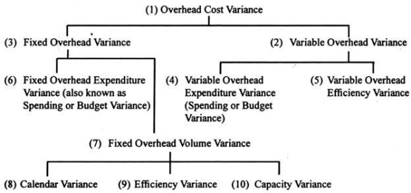
1) Total overhead difference:
Formula:
(Actual overhead incurred) – (Standard time of actual output x Standard overhead rate per hour)
Or
(Actual overhead incurred) – (Actual overhead x standard overhead rate per unit)
To explain the general overhead difference, the department's actual overhead cost was Rs 1, 00,000 in January, and therefore the standard (or allowed) time of the work performed was a complete of 4,500 hours, actually used. Suppose the time spent is 5,000 hours.
With an overhead rate of 20 Renault per hour, the general overhead difference is:
Actual department overhead | Rs 1,00,000 |
Overhead charged to production (4,500 hr × Rs 20) | Rs 90,000 |
Overall or et overhead variance (Unfavourable) | Rs 10,000 |
(2) Variable overhead difference:
This is the difference between the particular variable overhead and therefore the standard variable overhead allowed for the output actually achieved.
The formula for calculating this variance is:
(Actual variable overhead) – (Actual output x variable overhead per unit)
Or
(Actual variable overhead) – (Standard time of actual output x standard variable overhead per hour)
(3) Fixed overhead difference:
This difference is calculated using the subsequent formula:
Fixed Overhead Difference = (Actual Overhead – Absorption of Overhead)
Or
(Actual fixed overhead) – (Actual output x fixed overhead per unit)
Or
(Actual fixed overhead) – (Standard time of actual output x Standard fixed overhead per hour)
(4) Difference in variable overhead (expenditure or budget):
This difference shows the difference between actual variable overhead and budget variable overhead supported actual working hours.
This difference is detected using:
(Actual variable overhead – budget variable overhead)
(5) Difference in variable overhead efficiency:
This difference is analogous to the difference parturient efficiency and occurs when the particular working hours differ from the quality time required to supply an honest unit. Thanks to the high or low efficiency of workers engaged within the manufacture of products, actual production and standard fixed quantity may differ.
This difference is calculated using the subsequent formula:
(Actual time – civil time of actual output) x standard variable overhead rate per hour
(6) Difference in fixed overhead (expenditure or budget):
This difference shows the difference between the particular fixed overhead and therefore the budget fixed overhead.
The formula for calculating this variance is:
(Actual fixed overhead – budget overhead)
If the particular fixed overhead is bigger than the budget's fixed charge, the particular cost will exceed the budget, creating an unfavorable difference. Actual overhead costs are rarely adequate to budget costs, as fixed asset tax rates can change, premiums increase, and equipment changes can affect depreciation rates.
As an example, suppose a corporation completes 36,000 units (equivalent to a typical production time of 18,000) in 18,500 hours with a recorded fixed charge of Rs 7, 51,000. The quality fixed charge per hour is 40 rupees. Therefore,
Spending Difference = (Actual Fixed Overhead – Budget Overhead)
That is, = 7, 51,000 – (18,500 x 40)
= 7, 51,000 – 7, 40,000
= Rs 11,000 (undesirable)
Expenditure or budget variances provide management with information that helps them manage costs. Budget variances are typically created on a department-by-department basis, so department managers have control over the factors that cause budget variances.
(7) Fixed overhead volume difference:
Volume differences relate only to fixed overhead. This difference is between the quality fixed overhead allowed (absorbed) for the particular output and therefore the budget fixed overhead supported the quality time allowed for the particular output achieved during the amount. It’s caused by the difference. Differences indicate over absorption or under absorption of fixed overhead over a specific period of time. If the particular output is bigger than standard output, there's over absorption and fluctuations are favorable. Volume fluctuations aren't desirable if the particular output is a smaller amount than standard output.
The formula for calculating this variance is:
(Budget fixed overhead applied to actual output – Budget fixed overhead supported civil time allowed for actual output)
Or
(Actual production-budget production) x fixed overhead per standard unit
Volume distribution is further subdivided into three distributions.
(8) Differences in fixed overhead calendars:
This is the part of the quantity difference thanks to the difference between the particular working days of the amount to which the budget is applied and therefore the budget days of the budget period.
If the particular working days are longer than the budget working days, the difference is sweet because the work is completed quite the budget or allowed days. The reverse is additionally true.
The formula is:
(Actual working days – Budget working days) x Standard Fixed overhead rate per day. Calendar variances are often calculated supported time or output.
Then the formula is:
Time standard:
Calendar variance = (revised budget capacity time – budget time) x standard fixed overhead per hour
The difference is advantageous if the revised budget capacity time is bigger than the budget time. Within the opposite situation, the difference is at an obstacle.
Output standard:
Calendar variance = (Revised budget quantity for actual working days – Budget quantity) x Standard fixed overhead per unit
When the revised budget quantity is bigger than the budget quantity. Variance is advantageous. If the revised budget quantity is little, the variance is going to be at an obstacle.
(9) Difference in fixed overhead efficiency:
It is the quantity variance that happens when the particular production time used for the particular output differs from the quality time specified for that output. If the particular working hours are shorter than the quality time, the difference is advantageous, and if the particular time exceeds the quality time, the difference is disadvantageous.
The formula is:
Difference in fixed overhead efficiency = (actual time – civil time of actual production) x fixed overhead rate per hour
Fixed Overhead Efficiency Variance = (Actual Production – Standard Production by Actual Available Time) x Fixed Overhead Rate per Unit
(10) Difference in fixed overhead capacity:
This is a part of the fixed overhead volume difference thanks to the difference between the particular capacity (in hours) and therefore the budgeted capacity (expressed in hours) that ran during a specific period of time.
Ceremony Capacity variance = (actual capacity time – budget capacity) x standard fixed overhead rate per hour
This difference also represents idle time. If the particular capacity time is bigger than the budget capacity time, the difference is favorable, and if the particular capacity time is a smaller amount than the budget capacity time, the difference is disadvantageous.
If the particular and budgeted days also are specified, the budgeted capacity hours are calculated in actual days and are called the revised budgeted capacity hours, or actual working days budgeted hours.
In this case, the formula for calculating the capacitance difference is:
Capacity variance = (actual capacity time – revised budget capacity time) x standard fixed overhead rate per hour.
In the above formula, if the particular capacity time is bigger than the modified budget time, the difference is going to be advantageous. However, if the particular capacity time is shorter than the modified budget time, the difference is disadvantageous because it means the particular working hours are going to be reduced in consideration of the particular working days.
Two-way, three-way, and four-way ANOVA:
The above overhead variances also are categorized as two-way, three-way, and four-way differences.
The various differences between these categories are shown below:
(A) Two-way ANOVA:
Two-way ANOVA calculates two variance budget variances (sometimes called flexible budget or controllable variances) and volume variances. This suggests that:
(I) Budget differences = variable spending differences + fixed spending (budget) differences + fluctuating efficiency differences
(Ii) Volume distribution = Fixed volume distribution
(B) Three-way analysis of variance:
The three-way analysis calculates three variances: spending, efficiency, and volume. Therefore,
(I) Difference in expenditure = Difference in variable expenditure + Difference in fixed expenditure (budget)
(Ii) Efficiency distribution = Variable efficiency distribution
(Iii) Volume distribution = Fixed volume distribution
(C) 4-way analysis of variance:
The four-way analysis includes:
(I) Differences in fluctuating spending
(Ii) Difference in fixed expenditure (budget)
(Iii) Variable efficiency distribution
(Iv) Fixed volume fluctuation.
Example Problem
Department A will send the following data during the week ending October 31st:
Statement of department A fixed overhead variance:
Actual output (in units) | Rs 1,200 |
Standard hours | 40 |
Actual hours | 32 |
- Standard production per standard hour = Standard output/Standard hours
= 1,400/40 = 35 units
2. Standard fixed overhead rate per unit=Standard fixed overhead/Standard units produced
= Rs 1,40,000/1,400 = Rs 100
3. Standard fixed overhead rate per hour =Standard fixed overhead/Standard hours worked
= Rs 1,40,000/40 = Rs 3,500
A. Difference in spending:
(Actual overhead – budget overhead)
1, 50,000 rupees – 1, 40,000 rupees = 10,000 rupees (reverse)
B. Volume fluctuations:
Fixed overhead rate x per standard unit (actual output – budget output)
100 rupees (1,200 – 1,400) = 20,000 rupees (reverse)
C. Differences in total overhead costs:
(Actual overhead – overhead recovered by actual output)
Rupees 1, 50,000 – Rupees 1, 20,000 = Rupees 30,000 (reverse)
(A) Difference in efficiency:
Fixed overhead x per standard unit (actual production – standard production in actual time)
100 rupees (1200 – 32 x 35) = 8000 rupees (preferable)
 (B) Capacity difference:
Standard fixed overhead per hour (actual time – standard time)
3,500 rupees (32-40) = 28,000 rupees (reverse)
Gross profit analysis identifies the causes of changes in gross profit. Differences that affect gross profit are reported and corrective actions can be taken.
- Cause of profit difference
- Changes in unit sales price and cost
- Changes in sales volume
- Changes in sales composition
Change analysis provides the data you need to keep your production operations in line with your budget expectations. You need to compare this year's budget with actual operations, or between previous year's actual operations and this year's actual operations. Changes in gross profit can be seen for the entire company or by product line.
In order to improve profitability, it is important to change sales and sales composition as well as increase total sales. For example, if the total amount within your budget is constant, but you sell more profitable products than your budget, you will get higher profits. For example, in the furniture business, the quantity may not be very high, but there is a growing tendency for more expensive and durable margins per piece. Calculating and analyzing sales composition variances is a very important part of profit analysis. This provides additional insight into (a) why profits have increased or decreased compared to the previous year, and (b) why actual profits differed from what was originally expected.
Types of criteria in profit variance analysis
To identify the various causes of favorable or unfavorable fluctuations (increase) in profits, some criteria are needed to compare with actual results. The base may be based on the price and cost of the previous year, or any year selected as the base period. Some companies summarize profit variance analysis data in their annual reports by showing deviations from the reported revenues of the previous year.
However, you can establish more effective management and budgeting methods than the previous year's data. The combination of standards or budgets can be determined using advanced techniques such as linear and goal planning.
How to Calculate Profit Variance for a Single Product Company?
Profit variance analysis is the simplest for a single product company. This is because there is only one selling price, one set of costs (or cost prices), and a single sales volume. Disadvantageous profit variances can be categorized into four components: selling price variances, cost price variances, sales quantity variances, and cost quantity variances.
The difference in selling price measures the effect of a change in selling price on a company's contribution margin (or gross profit). This is calculated as follows:
Selling price difference = (actual price-budget price) x actual selling
For example, if the actual price is lower than the budget price, this difference is not desirable. It tends to reduce profits. However, cost variances are only a summary of price variances for materials, labor, and overhead costs. (This is the sum of the differences in material prices, labor rates, and factory overhead spending.) It is calculated as follows:
Cost variance = (actual cost – budget cost) x actual sales
For example, if the actual unit price is lower than the budget cost, this difference is beneficial. It tends to increase profits. Obtaining the difference in selling price minus the difference in cost simplifies the calculation of the difference in price, which is called the difference in gross margin per unit or the difference in contribution margin per unit.
Differences in sales volume indicate the impact of changes in unit sales on corporate profits. This is the amount that sales would have fluctuated from the budget if only the sales volume had changed. This is calculated as follows:
Sales quantity difference = (actual sales-budget sales) x budget price
This is an advantage if the actual sales volume is greater than the budget sales volume. It tends to increase profits. The difference in cost volume has the same interpretation. That is:
(Actual sales-budget sales) x budget cost per unit
The difference between the sales volume difference and the cost volume difference is called the "total volume difference".
How to calculate the variance of companies with multiple products?
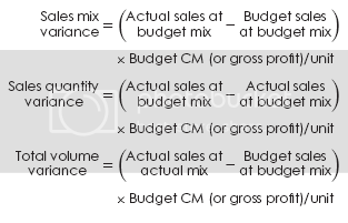
When a company produces multiple products, there is a fourth element of profit diversification. This is a difference in sales composition, which is the effect on profits of selling a product composition that is different from the budget. This difference occurs when different products have different contribution margins. For companies with multiple products, the actual sales volume may differ from your budget in two ways. Total unit sales may differ from your target total sales. In addition, the composition of the products actually sold may not be proportional to the target composition. Each of these two different types of changes in volume is reflected in the individual differences.
There are two types of total variance, sales composition variance and sales volume variance. The difference between these two should be used to evaluate the marketing department of the company. Differences in sales composition show how well a department has done in selling more profitable products and differences in sales volume measure how well a company has done in terms of overall sales volume. They are calculated as follows:
Problem 1:
Given to the factory:
100 regular workers
80 hours paid per week
Standard wage rate per hour Rs.1.60
Department standard output
40 units per hour considering normal idle time
In the first week of January 2003, it was confirmed that 2,000 units were produced and Rs 1.80 per hour were the actual wage, despite 20% of the idle time due to the power outage. Calculate labor variances.
Solution:
Standard Hours for actual output = 2,000 units × 100/40 units = 5,000 hours
Standard Labor Cost = 5,000 hours ×Rs. 1.60 = Rs. 8,000
Actual Hours = 100 ×80 = 8,000
Actual Labor Cost = 8,000 × 1.80 = Rs. 14,400
Idle Hours = 8,000 hrs. × 20/100 = 1,600
Actual Hours for Efficiency Variance = 8,000 – 1,600 = 6,400 hours.
Analysis of Labor Cost Variance
Labour Cost Variance | = (SLC – ALC) = Rs. 8,000 – Rs, 14,400 | Rs 6,400 (A) |
Explained by:
( SR – AR ) × AH |
( Rs. 1.60 – Rs. 1.80)8,000 = (-0.20) ×8,000) |
1,600 ( A) |
Ii. Labour Efficienecy Variance | (SH – AH) × SR (5,000 – 6,400 ) Rs. 1.60 |
2,240 ( A ) |
Iii. Idle Time Variance = Idle Hours × SR | = 1,600 × Rs. 1.60 | 2,560 ( A ) |
| ||
Problem 2:
From the following data, create a unit cost statement that shows the prime costs for products A and B with ANOVA.
| Product A | Product B |
Material : Standard | 6 kgs. @ RS. 5.00 | 90 kgs. @ RS. 3.00 |
Actual | 580 kgs. @ RS.5.500 | 100 kgs. @ RS. 2.50 |
Standard | 80 hours. @ RS.2.00 | 16 hours @ Rs. 2.50 |
Actual | 92 hours @ Rs 1.75 | 14 hours @ Rs. 2.60 |
Solution:
Variance
| Product A | Product B |
| = AQ × ( SP – AQ) = 580 × ( Rs. 5- Rs. 5.50) = 580 × 0.50 Rs. 290 (A) | = AQ × ( SP – AQ) = 100 × (3-2.80) = 100 × 0.20 = Rs. 20 (F) |
2. Material Usage Variance | (SQ-AQ) × Sp (600 kgs. – 580 kgs.) × 5 =(20) × 5 = 100 (F) | (SQ-AQ) SP (9—100) × Rs. 3 = RS. 30 (A) |
3. Material Cost Variance | (Price Variance – Usage Variance ) RS. 290 (a) – Rs. 100 (F) = RS 190 (A) | (Price Variance – Usage Variance) Rs. 20 (F) – 30 (A) = Rs. 10 (A) |
4. Labour Rate Variance | ( SR – AR ) × AH (Rs. 2- Rs. 1.75 ) × 92 = Rs. 190 (A) | ( SR – AR ) × AH (Rs. 2.80 – Rs. 2.60) × 14 = 0.20 × 14 hours = Rs. 2.80 (F)
|
5. Labour Efficiency Variance | ( SH – AH ) × SR ( 80 hours – 92 hours ) × Rs.2 = Rs. 24 (A)
| ( SH – AH ) × SR (16 – 14) × 28 = Rs. 5.60 (F)
|
6. Labour Cost Variance | Labour Rate Variance – Labour Efficiency Variance Rs. 23(F) – Rs. 24 (A) = Rs. 1.00 (A) | Labour Rate Variance + Labour Efficiency Variance Rs. 2.80 (F) + Rs. 5.60 (F) = Rs. 8.40 (F) |
Cost Statement
Product A |
| Product B |
|
| Rs |
| RS |
Material: 600 kgs. × Rs. 5.00 = | 3,000.00 | 90 kgs × Rs. 3.00 | 270.00 |
Labour: 80 hrs. × Rs 2.00 = | 160.00 | 16 hours × Rs. 2.80 = | 280.00 |
( A) Standard Prime Cost | 3160.00 |
| 314.80 |
Material: 580 kgs. × Rs. 5.50 = | 3,190 | 100 kgs × Rs. 2.80 | 280.00 |
Labour: 92 hours × Rs. 1.75 = | 161161 | 14 hours ×Rs. 2.60 | 316.40 |
(B) Actual Prime Cost | 3,351 |
| 316.40 |
Total Cost Variance = Rs. 3,160 – Rs. 3,351 = Rs 191.00 (A) | Rs. 314.80 – Rs. 316.40 = Rs 1.60 (A) | ||
Problem 3:
Worker gangs usually consist of 30 men, 15 women, and 10 boys. You will be paid at the standard hourly rate as follows:
Re
Men 0.80
Women 0.60
Boys 0.40
In a normal working week of 40 hours, the gang is expected to generate 2,000 units of output. During the week ending December 31, 2002, the gang consisted of 40 men, 10 women and 5 boys. Wages (daily expenses) paid were @ Re 0.70, Re 0.65 and Re 0.30, respectively. Due to an abnormal idle time, 4 hours were lost and 1,600 units were produced.
Calculation:
- Wage differences;
- Difference in wage rate;
- Differences in labor efficiency;
- Labor mix differences; and
- Difference in working idle time.
Solution:
Workers | Standard | Actual | ||||
| Hours | Rate (Rs.) | Amount Rs. | Hours | Rate | Amount Rs. |
Men | 1,200 | 0.80 | 960 | 1,600 | 0.70 | 1,120 |
Women | 600 | 0.60 | 360 | 400 | 0.65 | 260 |
Boys | 400 | 0.40 | 160 | 200 | 0.30 | 60 |
| 2,2oo |
| 1,480 | 2,200 |
| 1,440 |
- Labour Cost Variance = ( Actual Labour Cost – St. Labour Cost for Actual Output)
= Rs. 1,440 – (1,480/2,000)× 1,600 = Rs. 256 (A)
2. Wage Rate Variance = Actual Hours paid × ( Standard Rate – Actual Rate )
Rs.
Men = 1,600 × (0.80 – 0.70) = 160 (F)
Women = 400 × (0.60 -0.65) = 20 (A)
Boys = 200 × (0.30 – 0.40) = 20 (A)
3. Labour Efficiencey Variance = St. Rate × ( St. Hours – Actual Hours)
Men = 0.80 × [(1,600 × (1,200/2,000) – 1,600 ]
= 0.80 × (960 = 1,600) = Rs. 512 (A)
Women = 0.60 × [(600/2000) × 1,600) – 400]
= 0.60×(480 – 400 ) = 48 (F)
Boys = 0.40 × (400/2,000) × 1,600) – 200]
= o.40 × (320 – 200) = Rs. 48 (F)
4. Labour Mix Variance = St. Rate × (Actual time worked – Revised St.time)
Men = Re. 0.80 × (1,440 – 1,980×1,200/2,220)
= 0.80 × (1,440 – 1,080) = Rs. 288 (A)
Problem 4:
Calculate labor variance from the following data.
Total direct wage Rs.36, 000
Standard time generated 2,000
Standard rate per hour Rs.15
Actually paid time – Of the 1,800 hours, 50 hours are not working (abnormal idle time).
Solution:
- Labor Cost Variance = Standard cost of labor – Actual cost of labor
= (2,000 × Rs. 15) – (1,800 × 20)
= Rs. 30,000 – Rs. 36,000 = Rs. 6,000 (A)
Ii. Labor Rate Variance = Actual Time × (St. Rate – Actual Rate)
= 1,800 × (15 – 20) = Rs. 9,000 (A)
Iii. Labor Efficiency Variance = Standard Rate × (ST – AT)
= Rs. 15 × (2,000 – 1,750) = Rs. 3,750 (F)
Iv. Idle Time Variance = Abnormal Time × St. Rate
=50 × Rs. 15 = 750 (A)
Problem 5:
Calculate the variance overhead variance from the details below.
Actual variable overhead expense Rs. 14,250
Budgeted variable overhead expense RS. 17,000
Actual level of production 8,000 Standard hours
Normal capacity 10,000 Standard hours
Solution:
Variable Overhead Expenditure Variance = SC – AC
Standard Variable Overhead Expenses = Standard rate × Actual Output
Standard rate = Rs. 17,000/10,000 = Rs. 1.70.
So, Standard Variable Overhead Cost = 8,000 × Rs. 1.70 = Rs. 13,600
Therefore, Variable Overhead Cost Variance = SC – AC = Rs. 13,600 = Rs. 14,250
= 650 (Advance)
Problem 6:
Standard costing of manufacturing concerns includes the following details:
– 2 hours @ 0-30p. Per hour = 0-60p per unit .Variable overhead
Actual operating time 8,000 hours
Actual variable overhead Rs.2, 600
Actual production is 4,850 units
Calculate the required cost variance.
Solution:
We shall have to find out standard quantity and actual rate
Standard Quantity = Actual operating hours/Standard hours per unit = 8,000/2 = 4,000 units
Actual Rate = Actual overhead cost/Standard hrs.worked = Rs 2,600/4,000 = 0.65 p.
- Variable overhead cost variance = SC- AC
Standard Cost = Actual Qnt. × S.R = 4,850 × 0.60 p = Rs. 2,190
Variable overhead cost variance = Rs. 2,190 – Rs, 2,600 = 310 (F)
Ii. Variable overhead cost variance = Standard unit× (SR – AR)
= 4,000 × (0.60 – 0.65) = Rs. 200 (A)
Iii. Variable overhead efficiency variance = SR × (AQ – SQ)
= 0.60 p × (4,850 – 4,000) = Rs. 510 (F)
Problem 7:
Calculate from the following details.
(a) Material cost variance
(b) Material price variance
(c) Material usage variance
Quantity of material purchased 3000 units
Value of material purchased Rs. 9,000
Standard quantity of material
Required per ton of output 30 units
Standard rate of material Rs. 2.50 per unit
Opening stock of material Nil
Closing stock of material 500 units
Output during the year 80 tons
Solutions:
(a) Quantity of material consumed : 3,000 units – 500 units = 2,500 units
(b) Actual cost of material per unit = Rs. 9,000/3,000 = Rs. 3
(c) Standard material required per ton 30 units
(d) Standard material cost = 30 × 80 × Rs. 2.50 = 2,400 × 2.50 = Rs. 6,000
Actual cost = 2,500 × Rs. 3 = Rs. 7,500
(i) Material Cost Variance = SC- AC
= Rs. 6,000 – Rs. 7,500 = Rs. 1,500 (A)
(ii) Material Price Variance = AQ × (SR – AR)
= 2,500 × (2.50 – 3.00) = R. 1,250 (A)
(iii) Material usage Variance = SR × (SQ – AQ)
= Rs. 2.50 × (2,400 – 2,500)
= Rs. 2.50 × (-100) = 250 (A)
Reconciliation
MCV = MPV + MUV = 1,500 (A) = 1,250 (A) + 250 (A)
References:
- Https://bbamantra.com/standard-costing/
- Https://www.yourarticlelibrary.com/accounting/standard-costing/standard-costing-meaning-objectives-advantages-and-disadvantages/66374
- Https://courses.lumenlearning.com/sac-managacct/chapter/advantages-and-disadvantages-of-standard-costing/#:~:text=A%20standard%20cost%20system%20can,identical%20products%20may%20differ%20widely.
- Https://www.indeed.com/career-advice/career-development/standard-costing-definition
- Https://freebcomnotes.blogspot.com/2017/07/standard-costing-meaning-advantages-and.html
- Https://hmhub.me/types-variance-cost-material-labour-overheadfixed-overhead-sales-profit/