Unit-3
Summarization Measures
A measure of central tendency is a single value that attempts to describe a set of data by identifying the central position within that set of data. As such, measures of central tendency are sometimes called measures of central location.
Terms for statistics
- Population: Any well-defined set of objects about which a statistical inquiry is being made is the population. The information required from each individual member of the population is called its characteristic.
- Variate and attribute: if the characteristic that is being studied is numerical then it is called variate. The qualitative characteristic under study is called attribute
- Discrete variable: A variate which takes only integer values, like 1, 2, 3, …. 10,100, even 0, -2,-5 etc. will come under a discrete variate
- Continuous variate: A variate which is capable of taking all the values is called continuous values.
- Data in statistics: when the characteristic under study of a population is collected, it is called data.
- Frequency distribution: if instead of 10 students, we have 100 students then frequency is better choice to handle this data, frequency will give number of times the relevant variate
- Cumulative Frequencies: for each value x of a variate, we can speak of the total number of observations less than or equal to x, within its range.
- Arithmetic mean (A.M):It is mean or the average value.
Average or measures of Central tendency
Professor Bowley defines the average as-
“Statistical constants which enable us to comprehend in a single effort the significance of the whole”
An average is a single value that is the best representative for a given data set.
Measures of central tendency show the tendency of some central values around which data tend to cluster.
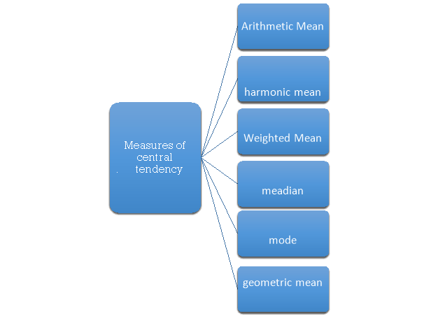
The following are the various measures of central tendency-
1. Arithmetic mean,
2. Median,
3. Mode,
4. Weighted mean,
5. Geometric mean,
6. Harmonic mean.
The arithmetic mean or mean-
The arithmetic mean is a value which is the sum of all observation divided by a total number of observations of the given data set.
If there are n numbers in a dataset-  then the arithmetic mean will be-

If the numbers along with frequencies are given then mean can be defined as-

This is known as direct method.
Example: Find the mean of 20, 22, 25, 28, 30.
Sol:

Example: Find the mean of 26, 15, 29, 36, 35, 30, 14, 21, 25 .
Sol.


Example: Find the mean of the following:
Numbers | 8 | 10 | 15 | 20 |
Frequency | 5 | 8 | 8 | 4 |
Sol:
 fx = 8×5 + 10×8 + 15×8 + 20×4 = 40+80+120+80=320
 f = 5+8+8+4=25
A.M.= 
Example: Find the mean of the following dataset.
x | 20 | 30 | 40 |
f | 5 | 6 | 4 |
Sol.
We have the following table-
X | F | Fx |
20 | 5 | 100 |
30 | 6 | 180 |
40 | 7 | 160 |
| Sum = 15 | Sum = 440 |
Then Mean will be-


(b) Short cut method
Let a be the assumed mean, d the derivation of the variate x from a. Then


Example: Find the arithmetic mean for the following distribution
Class | 0-10 | 10-20 | 20-30 | 30-40 | 40-50 |
Frequency | 7 | 8 | 20 | 10 | 5 |
Sol:
Let assumed mean (a) = 25
Class | Mid-value (x) | Frequency (f) |  | Fd |
0-10 | 5 | 7 | -20 | -140 |
10-20 | 15 | 8 | -10 | -80 |
20-30 | 25 | 20 | 0 | 0 |
30-40 | 35 | 10 | + 10 | +100 |
40-50 | 45 | 5 | + 20 | +100 |
Total |
| 50 |
| -20 |

(C) Step deviation method
Let a be the assumed mean, i the width of the class interval and

Example:
Find the arithmetic mean of the data given in above example 3 by step deviation method.
Solution. Let a =25
Class | Mid-value x | Frequency F |  | f.D |
0-10 | 5 | 7 | -2 | -14 |
10-20 | 15 | 8 | -1 | -8 |
20-30 | 25 | 20 | 0 | 0 |
30-40 | 35 | 10 | +1 | +10 |
40-50 | 45 | 5 | +2 | +10 |
Total |
| 50 |
| -2 |

Median
Median is defined as the measure of the central atom when they are arranged in ascending or descending order of magnitude.
Median is the mid-value of the given data when it is arranged in ascending or descending order.
1. If the total number of values in the data set is odd then the median is the value of  item.
item.
2. If the total number of values in the data set is even then the median is the mean of the  item.
item.
Note- The data should be arranged in ascending or descending order
Example:
Find the median of 6, 8, 9, 10, 11, 12, 13.
Sol:
Total number of items =7
The middle item 
Median= value of the 4th item = 10
Example: Find the median of the data given below-
7, 8, 9, 3, 4, 10
Sol.
Arrange the data in ascending order-
3, 4, 7, 8, 9, 10
So there total 6 (even) observations, then-


=
Median for grouped data-

Here,


Example 6. Find the value of median from the following data
Number of days for which absent (less than) | 5 | 10 | 15 | 20 | 25 | 30 | 35 | 40 | 45 |
Number of students | 29 | 224 | 465 | 582 | 634 | 644 | 650 | 653 | 655 |
Solution. The given cumulative frequency distribution will first be converted into ordinary frequency as under:
Class interval | Cumulative frequency | Ordinary frequency |
0-5 | 29 | 29=29 |
5-10 | 224 | 224-29=105 |
10-15 | 465 | 465-224=241 |
15-20 | 582 | 582-465=117 |
20-25 | 634 | 634-582=52 |
25-30 | 644 | 644-634=10 |
30-35 | 650 | 650-644=6 |
35-40 | 653 | 653-650=3 |
40-45 | 655 | 655-653=2 |
Median = size of 
327.5th item lies in 10-15 which is the median class

Where l stands for lower limit of median class.
N stands for the total frequency
C stands for cumulative frequency just preceding the median class
i stands for class interval
f stands for frequency for the median class


Example: Find the median of the following dataset-

Sol.
Class interval | Frequency | Cumulative frequency |
0 - 10 | 3 | 3 |
10 – 20 | 5 | 8 |
20 – 30 | 7 | 15 |
30 – 40 | 9 | 24 |
40 – 50 | 4 | 28 |

So that median class is 20-30.
Now putting the values in the formula-


So that the median is 28.57
Mode
Mode is defined to be the size of the variable which occurs most frequently.
Example:
Find the mode of the following items
0,1,6,7,2,3,7,6,6,2,6,0,5,6,0.
Sol:
6 occurs 5 times and no other item occurs 5 or more than 5 times, hence the mode is 6.
Mode for grouped data-

Here,


Empirical formula
Mean – Mode =3 [Mean – Median]
Example: Find the mode from the following data
Age | 0-6 | 6-12 | 12-18 | 18-24 | 24-30 | 30-36 | 36-42 |
Frequency | 6 | 11 | 25 | 35 | 18 | 12 | 6 |
Solution.
Age | Frequency | Cumulative frequency |
0-6 | 6 | 6 |
6-12 | 11 | 17 |
12-18 |  | 42 |
18-24 | 35 = f | 77 |
24-30 |  | 95 |
30-36 | 12 | 107 |
36-42 | 6 | 113 |


Example: Find the mode of the following dataset-

Sol.
Class interval | Frequency |
0 - 10 | 3 |
10 – 20 | 5 |
20 – 30 | 7 |
30 – 40 | 9 |
40 – 50 | 4 |
Here the highest frequency is 9. So that the modal class is 40-50,
Put the values in the given data-


Hence the mode is 42.86
Example: A survey was conducted in a housing complex, to find out numbers of person in various age groups, who are using the ATM cards of banks. The result of the survey are as shown below.
Age group | Number of persons |
Below 20 | 10 |
Below 40 | 25 |
Below 60 | 50 |
Below 80 | 70 |
Find the mode of above distribution
Solution:
Class interval | Frequencies |
0-20 | 10 |
20-40 | 25-10=15 |
40-60 | 50-25=25 |
60-80 | 70-50=20 |
The maximum frequency 25 is for the class 40-60
Class 40-60 is modal class.
By using formula-

We get-
Mode = 53.3333
Example:
Calculate the value of modal worker family’s monthly income from the following data: | |||||||||||||||||||||||||||||||||||||||||||||||||||||||
Less than cumulative frequency distribution Of income per month (in ‘000 Rs) | |||||||||||||||||||||||||||||||||||||||||||||||||||||||
| |||||||||||||||||||||||||||||||||||||||||||||||||||||||
|
Sol: | ||||||||||||||||||||||||||||||||||||||||||||||||||||||
| This table should be converted into an ordinary frequency Table to determine the modal class. | ||||||||||||||||||||||||||||||||||||||||||||||||||||||
|
| ||||||||||||||||||||||||||||||||||||||||||||||||||||||
|
The value of the mode lies in 25–30 class interval. By inspection also, it can be seeming that this is a modal class. Now L =25, D1 (30–18) = 12, D2 = (30-20) =10, h = 5 Using the formula, you can obtain the value of the mode as: | ||||||||||||||||||||||||||||||||||||||||||||||||||||||
| 

| ||||||||||||||||||||||||||||||||||||||||||||||||||||||
| Thus, the modal worker family’s monthly income is Rs 27.273. | ||||||||||||||||||||||||||||||||||||||||||||||||||||||
Geometric mean
If  be n values of variates x, then the geometric mean

Example: Calculate the harmonic mean of 4,8,16.
Sol:


Note-
1. 
2. 
3. Mean – Mode = [Mean - Median]
Key takeaways-

- A measure of central tendency is a single value that attempts to describe a set of data by identifying the central position within that set of data.
- An average is a single value that is the best representative for a given data set.


- 2.

- 3. Mean – Mode = [Mean - Median]
Partition values-
The values divide the distribution into certain number of equal parts are called partition values.
Data should be arranged in ascending order descending order.
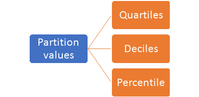
Quartile, deciles and percentile are the partition values.
Note-
- Quartile divides the data into four equal parts.
- Deciles and percentiles divide the distribution into ten and hundred equal parts, respectively
Quartile-
There are three quartiles, i.e. Q1, Q2 and Q3 which divide the total data into four equal parts when it has been orderly arranged. Q1, Q2 and Q3 are termed as first quartile, second quartile and third quartile or lower quartile, middle quartile and upper quartile, respectively. The first quartile, Q1, separates the first one-fourth of the data from the upper three fourths and is equal to the 25th percentile. The second quartile, Q2, divides the data into two equal parts (like median) and is equal to the 50th percentile. The third quartile, Q3, separates the first three-quarters of the data from the last quarter and is equal to 75th percentile.
For ungrouped data, we find the quartiles as follows-


For grouped data, we find the quartiles as follows-
i’th quartile can be find as-

l = lower class limit of i'th quartile class,
h = width of the ith quartile class,
N = total frequency,
C = cumulative frequency of pre ith quartile class, and
f = frequencies of ith quartile class.
Deciles
Deciles divide whole distribution in to ten equal parts. There are nine deciles.
For ungrouped data, we find the deciles as follows-

For grouped data, we find the deciles as follows-
i’th decile can be find as-

Percentile-
Percentiles divide whole distribution in to 100 equal parts. There are ninety nine percentiles.
For ungrouped data, we find the percentile as follows-

For grouped data, we find the percentile as follows-
i’th percentile can be find as-

Example: Calculate the first and third quartile of the following data-
Class interval | f |
0-10 | 3 |
10-20 | 5 |
20-30 | 7 |
30-40 | 9 |
40-50 | 4 |
Sol.
Class interval | f | CF |
0-10 | 3 | 3 |
10-20 | 5 | 8 |
20-30 | 7 | 15 |
30-40 | 9 | 24 |
40-50 | 4 | 28 |
| N = 28 |
|
Here N/4 = 28/4 = 7
The 7th observation falls in the class 10-20. So, this is the first quartile class. 3N/4 = 21th observation falls in class 30-40, so it is the third quartile class.
For first quartile l = 10, f = 5, C = 3, N = 28
We know that-


For third quartile l = 30, f = 9, C = 15

Concept of Ogive-
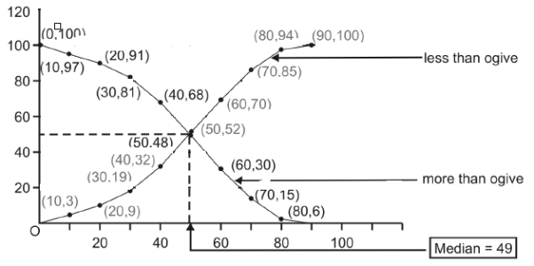
For drawing less than cumulative frequency curve (or less than ogive), first of all the cumulative frequencies are plotted against the values (upper limits of the class intervals) up to which they correspond and then we simply join the points by line segments, curve thus obtained is known as less than ogive. Similarly, more than frequency curve (more than ogive) can be obtained by plotting more than cumulative frequencies against lower limits of the class intervals. As we have already mentioned within brackets that less than cumulative frequency curve and more than cumulative frequency curve are also called less than ogive and more than ogive respectively.
We can define as follows-
Less Than Ogive: If we plot the points with the upper limits of the classes as abscissae and the cumulative frequencies corresponding to the values less then the upper limits as ordinates and join the points so plotted by line segments, the curve thus obtained is nothing but known as “less than cumulative frequency curve” or “less than ogive”.
More Than Ogive: If we plot the points with the lower limits of the classes as
Abscissae and the cumulative frequencies corresponding to the values more than the lower limits as ordinates and join the points so plotted by line segments, the curve thus obtained is nothing but known as “more than cumulative frequency curve” or “more than ogive”.
Note-
Median may also the obtained by drawing dotted vertical line through the point of inter section of both the ogives, when drawn on a single figure.
Example: By drawing ogive, find the median of the following data-
Class | 0-10 | 10-20 | 20-30 | 30-40 | 40-50 | 50-60 | 60-70 | 70-80 | 80-90 |
Frequency | 3 | 6 | 10 | 13 | 20 | 18 | 15 | 9 | 6 |
Sol:
Key takeaways-
- The values divide the distribution into certain number of equal parts are called partition values.
- Quartile divides the data into four equal parts.


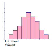
The highest peak of the histogram represents the location of the mode of the data set. The mode is the data value that occurs the most often in a data set. For a symmetric histogram, the values of the mean, median, and mode are all the same and are all located at the centre of the distribution.
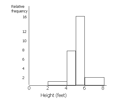
Draw a histogram for the following information.
Height (feet): | Frequency | Relative Frequency |
0-2 | 0 | 0 |
2-4 | 1 | 1 |
4-5 | 4 | 8 |
5-6 | 8 | 16 |
6-8 | 2 | 2 |
When drawing a histogram, the y-axis is labelled 'relative frequency' or 'frequency density'. You must work out the relative frequency before you can draw a histogram. To do this, first you must choose a standard width of the groups. Some of the heights are grouped into 2s (0-2, 2-4, 6-8) and some into 1s (4-5, 5-6).
Most are 2s, so we shall call the standard width 2. To make the areas match, we must double the values for frequency which have a class division of 1 (since 1 is half of 2). Therefore, the figures in the 4-5 and the 5-6 columns must be doubled. If any of the class divisions were 4 (for example if there was a 8-12 group), these figures would be halved. This is because the area of this 'bar' will be twice the standard width of 2 unless we half the frequency.
Area of bar = frequency x standard width
The arithmetic mean denoted x, of a set of n numbers x1, x2, …, xn is defined as the sum of the numbers divided by n:
The arithmetic mean (usually synonymous with average) represents a point about which the numbers balance. For example, if unit masses are placed on a line at points with coordinates x1, x2, …, xn, then the arithmetic mean is the coordinate of the centre of gravity of the system.
Example: A student obtained the marks 40, 50, 60, 80, and 45 in math, statistics, physics, chemistry and biology respectively. Assuming weights 5, 2, 4, 3, and 1 respectively for the above-mentioned subjects, find the weighted arithmetic mean per subject.
Solution: | Mark Obtained | Weight | Wxwx |
Math | 4040 | 55 | 200200 |
Statistics | 5050 | 22 | 100100 |
Physics | 6060 | 44 | 240240 |
Chemistry | 8080 | 33 | 240240 |
Biology | 4545 | 11 | 4545 |
Total |
| ∑w=15∑w=15 | ∑wx=825∑wx=825 |
Now we will find the weighted arithmetic mean as:
Xw=∑wx∑w=82515=55X
w=∑wx∑w=82515=55 marks/subject.
Example: Suppose that a marketing firm conducts a survey of 1,000 households to determine the average number of TVs each household owns. The data show a large number of households with two or three TVs and a smaller number with one or four. Every household in the sample has at least one TV and no household has more than four.
Solution:
Here’s the sample data for the survey:
Number of TVs per Household | Number of Households |
1 | 73 |
2 | 378 |
3 | 459 |
4 | 90 |
As many of the values in this data set are repeated multiple times, you can easily compute the sample mean as a weighted mean. Follow these steps to calculate the weighted arithmetic mean:
Step 1: Assign a weight to each value in the dataset:
x1=1,w1=73
x2=2,w2=378
x3=3,w3=459
x4=4,w4=90
Step 2: Compute the numerator of the weighted mean formula.
Multiply each sample by its weight and then add the products together:
= =w1x1+w2x2+w3x3+w4x4
= (1)(73)+(2)(378)+(3)(459)+(4)(90)
=2566
Step 3: Now, compute the denominator of the weighted mean formula by adding the weights together.
= =w1+w2+w3+w4
= 73 + 378 + 459 + 90
=1000
Step 4: Divide the numerator by the denominator
= / wi
/ wi
=2566/1000
=2.566
The mean number of TVs per household in this sample is 2.566.
As the name suggests, the measure of dispersion shows the scatterings of the data. It tells the variation of the data from one another and gives a clear idea about the distribution of the data. The measure of dispersion shows the homogeneity or the heterogeneity of the distribution of the observations.
According to Spiegel, the degree to which numerical data tend to spread about an average value is called the variation or dispersion of data.
Classification of Measures of Dispersion
There are two basic kinds of a measure of dispersion-
- Absolute measures,
- Relative measures.
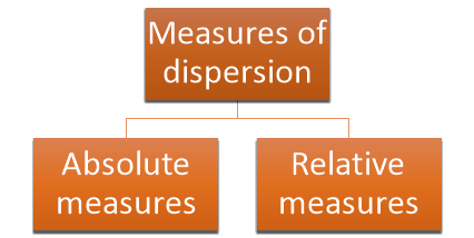
Following are the different types of measures of dispersion-
According to Spiegel-
“The degree to which numerical data tend to spread about an average value is called the variation or dispersion of data”
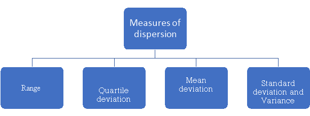
The different measures of dispersion are-
1. Range,
2. Quartile deviation,
3. Mean deviation,
4. Standard deviation
5. Variance.
Significance of measures of dispersion-
Measures of variation are pointed out as to how far an average is representative of the entire data. When variation is less, the average closely represents the individual values of the data and when variation is large; the average may not closely represent all the units and be quite unreliable.
Another purpose of measuring variation is to determine the nature and causes of variations in order to control the variation itself. Measurements of dispersion are helpful to control the causes of variation.
Many powerful statistical tools in statistics such as correlation analysis, the testing of hypothesis, the analysis of variance, techniques of quality control, etc. are based on different measures of dispersion.
Range is the simplest measure of dispersion. Range is the difference between the maximum value of the variable and the minimum value of the variable in the distribution.

Example: Find the range of the distribution 4, 22, 14, 12, 16, 8, 13, 17, 21, 6, 5, 26.
Sol.
For the given distribution, the maximum value is 26 and the minimum value is 4, so that the range of the distribution is –

Example- Find the range of the data- 8, 5, 6, 4, 7, 10, 12, 15, 25, 30
Sol. Here the maximum value is 30 and the minimum value is 4 so that the range is-
30 – 4 = 26
Coefficient of range-
The coefficient of range can be calculated as follows-
Coefficient of Range = 
Advantages of range-
- It is very simple to calculate
- It has useful applications in areas like order statistics and statistical quality control.
Disadvantages of range-
- It utilizes only the maximum and the minimum values of variable in the series and gives no importance to other observations
- It is affected by fluctuations of sampling
- If a single value lower than the minimum or higher than the maximum is added or if the maximum or minimum value is deleted range is seriously affected
The quartiles divide a data set into quarters. The first quartile, (Q1) is the middle number between the smallest number and the median of the data. The second quartile, (Q2) is the median of the data set. The third quartile, (Q3) is the middle number between the median and the largest number.
Quartile deviation or semi-inter-quartile deviation is

Relative measure of Q.D. Known as Coefficient of Q.D. And is defined as

Example: Find the quartile deviation of the following data.
Class interval | 0-10 | 10-20 | 20-30 | 30-40 | 40-50 |
Frequency | 3 | 5 | 7 | 9 | 4 |
Sol.
We have N/4 = 28/4 = 7 and 7th observation falls in the class 10-20.
This is the first quartile class. Similarly, 3N/4 = 21 and 21st observation falls in the interval 30-40. This is the third quartile class.
Class interval | f | CF |
0-10 | 3 | 3 |
10-20 | 5 | 8 |
20-30 | 7 | 15 |
30-40 | 9 | 24 |
40-50 | 4 | 28 |
| N = 28 |
|
By using the formula of quartile deviation, we will find  -
-


Therefore-
Q = ½ × (Q3 – Q1) = (36.67 – 18) / 2 = 9.335
Example: Find the quartile deviation of the following data-
Class | 0-5 | 5-10 | 10-15 | 15-20 | 20-25 | 25-30 | 30-35 | 35-40 |
Frequency | 6 | 8 | 12 | 24 | 36 | 32 | 24 | 8 |
Sol.
We will construct the cumulative frequency table-
Class interval | f | CF |
0-5 | 6 | 6 |
5-10 | 8 | 14 |
10-15 | 12 | 26 |
15-20 | 24 | 50 |
20-25 | 36 | 86 |
25-30 | 32 | 118 |
30-35 | 24 | 142 |
35-40 | 8 | 150 |
| N = 150 |
|
We know that-

So that

And

Therefore-
Q = ½ × (Q3 – Q1) = (30.52 – 17.40) / 2 = 6.56
Key takeaways-
- The measure of dispersion shows the homogeneity or the heterogeneity of the distribution of the observations.
- The degree to which numerical data tend to spread about an average value is called the variation or dispersion of data.

Mean deviation is the average of the sum of the absolute values of deviation from any arbitrary value viz. Mean, median, mode, etc.
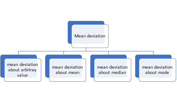 The deviation of an observation xi from the assumed mean A is defined as (xi – A).
Therefore,
The mean deviation can be defined as-

Mean deviation from mean is defined as-

Mean deviation from median is defined as-

For frequency distribution-


Example: Find the mean deviation from mean of the following data-

Sol.
x | F | Fx | |x-  | f|x-  |
1 | 3 | 3 | 3.24 | 9.72 |
2 | 5 | 10 | 2.24 | 11.20 |
3 | 8 | 24 | 1.24 | 9.92 |
4 | 12 | 48 | 0.24 | 2.88 |
5 | 10 | 50 | 0.76 | 7.60 |
6 | 7 | 42 | 1.76 | 12.32 |
7 | 5 | 35 | 2.76 | 13.80 |
Total | 50 | 212 | 12.24 | 67.44 |

We know that-

Example: The students of statistics got the marks as below-
16, 24, 13, 18, 15, 10, 23
Find the mean deviation from mean.
Sol.
X | x-17 | |x-  |
16 | -1 | 1 |
24 | 7 | 7 |
13 | -4 | 4 |
18 | 1 | 1 |
15 | -2 | 2 |
10 | -7 | 7 |
23 | 6 | 6 |
Sum = 119 |
| 28 |
Then

Hence

Example 11. Find the mean deviation of the following frequency distribution
Class | 0-6 | 6-12 | 12-18 | 18-24 | 24-30 |
Frequency | 8 | 10 | 12 | 9 | 5 |
Solution. Let a = 15
Class | Mid-value x | Frequency f | d = x-a | Fd | |x-14| | f|x-14| |
0-6 | 3 | 8 | -12 | -96 | 11 | 88 |
6-12 | 9 | 10 | -6 | -60 | 5 | 50 |
12-18 | 15 | 12 | 0 | 0 | 1 | 12 |
18-24 | 21 | 9 | +6 | 54 | 7 | 63 |
24-30 | 27 | 5 | +12 | 60 | 13 | 65 |
Total |
| 44 |
| -42 |
| 278 |

Then mean deviation from mean-

Key takeaways-
Variance-
Variance is the average of the square of deviations of the values taken from mean. Taking a square of the deviation is a better technique to get rid of negative deviations.
Variance is given as-

And for a frequency distribution, the formula is

Variance of the combined series-
If σ1, σ2 are two standard deviations of two series of sizes n1 and n2 with means ȳ1 and ȳ2. The variance of the two series of sizes n1 + n2 is:
σ 2 = (1/ n1 + n2) ÷ [n1 (σ1 2 + d1 2) + n2 (σ2 2 + d2 2)]
Where, d1 = ȳ 1 −ȳ , d2 = ȳ 2 −ȳ , and ȳ = (n1 ȳ 1 + n2 ȳ 2) ÷ ( n1 + n2).
Coefficient of variation
Coefficient of variation can be calculated as-

Note- The lower value of C.V, the more constancy of data
Example- If student A has a mean 50 with SD 10.Another student B has a mean of 30 with SD = 3.
Which one is the best performer?
Sol. We calculate C.V.-


And

Here B has a lower C.V. So that student B is the best performer.
Example: Calculate coefficient variation for the following frequency distribution.
Wages in Rupees earned per day | 0-10 | 10-20 | 20-30 | 30-40 | 40-50 | 50-60 |
No. Of Labourers | 5 | 9 | 15 | 12 | 10 | 3 |
Solution:
We already calculated

Now,
A.M 

A.M 
 Coefficient of Variation


Example: Suppose batsman A has mean 50 with SD 10. Batsman B has mean 30 with SD 3. What do you infer about their performance?
Sol.
A has higher mean than B. This means A is a better run maker.
However, B has lower CV (3/30 = 0.1) than A (10/50 = 0.2) and is consequently more consistent.
Note-
It is a relative measure of variability. If we are comparing the two data series, the data series having smaller CV will be more consistent.
Standard deviation-
It is defined as the positive square root of the arithmetic mean of the square of the deviation of the given values from their arithmetic mean. It is denoted by the symbol  .
.

Where  is A.M of the distribution
  . We have more formulae to calculate the standard deviation.


 ..
.. 
In frequency distribution from, we put  where H is generally taken as width of class interval


Shortcut formula to calculate standard deviation-

The square of the standard deviation is called known as a variance.

Example: Find the Variance and Standard Deviation of the Following Numbers: 1, 3, 5, 5, 6, 7, 9, 10.
Sol.
The mean = 46/ 8 = 5.75
Step 1: (1 – 5.75), (3 – 5.75), (5 – 5.75), (5 – 5.75), (6 – 5.75), (7 – 5.75), (9 – 5.75), (10 – 5.75)
= -4.75, -2.75, -0.75, -0.75, 0.25, 1.25, 3.25, 4.25
Step 2: Squaring the above values we get, 22.563, 7.563, 0.563, 0.563, 0.063, 1.563, 10.563, 18.063
Step 3: 22.563 + 7.563 + 0.563 + 0.563 + 0.063 + 1.563 + 10.563 + 18.063
= 61.504
Step 4: n = 8, therefore variance (σ2) = 61.504/ 8 = 7.69
Now, Standard deviation (σ) = 2.77
Example: Suppose a series of 100 data points has mean 50 and variance 20. Another series of 200 data points has mean 80 and variance 40. What is the combined variance of the given series?
Sol.
The mean of the combined series-

Therefore, d1= 50 – 70 = –20 and d2 = 80 – 70 =10
Variance of the combined series


Example: Find the standard deviation for the following numbers:
10, 27, 40, 60, 33, 30, 10
Sol.
First we prepare the following distribution table
X |  |
10 | 100 |
27 | 729 |
40 | 1600 |
60 | 3600 |
33 | 1089 |
30 | 900 |
10 | 100 |
Sum = 210 | 8118 |
Then-
Mean = 210 / 7 = 30
And standard deviation-


Example-1: Compute the variance and standard deviation.
Class | Frequency |
0-10 | 3 |
10-20 | 5 |
20-30 | 7 |
30-40 | 9 |
40-50 | 4 |
Sol.
Class | Mid-value (x) | Frequency (f) |  |
0-10 | 5 | 3 | 1470.924 |
10-20 | 15 | 5 | 737.250 |
20-30 | 25 | 7 | 32.1441 |
30-40 | 35 | 9 | 555.606 |
40-50 | 45 | 4 | 1275.504 |
Sum |
|  | 4071.428 |

Then standard deviation,

Example-2: Calculate the standard deviation of the following frequency distribution-
Weight | 60 – 62 | 63 – 65 | 66 – 68 | 69 – 71 | 72 – 74 |
Item | 5 | 18 | 42 | 27 | 8 |
Sol.
Weight | Item (f) | X | d = x – 67 | f.d |  |
60 – 62 | 5 | 61 | -6 | -30 | 180 |
63 – 65 | 18 | 64 | -3 | -54 | 162 |
66 – 68 | 42 | 67 | 0 | 0 | 0 |
69 – 71 | 27 | 70 | 3 | 81 | 243 |
72 – 74 | 8 | 73 | 6 | 48 | 288 |
Total |
100 |
|
|
45 |
873 |


Example: Calculate S.D for the following distribution.
Wages in rupees earned per day | 0-10 | 10-20 | 20-30 | 30-40 | 40-50 | 50-60 |
No. Of Labourers | 5 | 9 | 15 | 12 | 10 | 3 |
Solution:
Wages earned C.I | Mid value  | Frequency |  |  |  |
52 | 5 | 5 | -2 | -10 | 20 |
153 | 15 | 9 | -1 | -9 | 9 |
25 | 25 | 15 | 0 | 0 | 0 |
35 | 35 | 12 | 1 | 12 | 12 |
45 | 45 | 10 | 2 | 20 | 40 |
55 | 55 | 3 | 3 | 9 | 27 |
Total | - |  |  |  |  |
Using formula,


Key takeaways-
- Range = Max. Value – Min. Value
- Coefficient of Range =


References-
- Mathematics and Statistics for Business – R. S. Bhardwaj – Excel Books.
- Business Mathematics and Statistics – Subhanjali Chopra – Pearson publication.
- Fundamentals of Business Mathematics and Statistics – ICAI – ICAI.
- Business Mathematics and Statistics – Dr. J K Das, N Das – McGraw Hill Education.
- Mathematical and statistical techniques, Dr. Abhilasha S. Magar & Manohar B. Bhagirath
- IGNOU

