3.1 The IS-LM model of integration of commodity and money markets

The goods and the money markets are interlinked by two economic variables, namely: interest rate and national income. In this model, interest rate is introduced in the goods market through investment demand. The goods market therefore has two variables – interest rate (i) and national income (GDP). The goods market equation is known as the IS curve. The IS curve represents equality between saving (S) and investment (I) and all points on the IS curve show goods market equilibrium at different levels of interest and national income. The money market equilibrium is determined by the demand for and supply of money at various levels of interest and national income. The demand for money is a function of income and interest rate. The supply of money is determined by the Central Bank (the RBI in India or the Federal Reserve in the USA). The money market equation is known as the LM curve. The LM curve represents equilibrium between demand and supply of money at various levels of interest rates and national income. Various points on the LM curve shows equality between demand for money (L) and supply of money (M).

The IS-LM model shows how the equilibrium levels of income and interest rates are simultaneously determined by the simultaneous equilibrium in the two interdependent goods and money markets. Hicks, Hansen and Johnson put forward the IS-LM model on the basis of Keynesian framework of national income determination in which investment, national income, rate of interest, demand for and supply of money are interrelated and inter– dependent. These variables are represented by two curves, namely; the IS and the LM curves.

The goods market and the IS curve

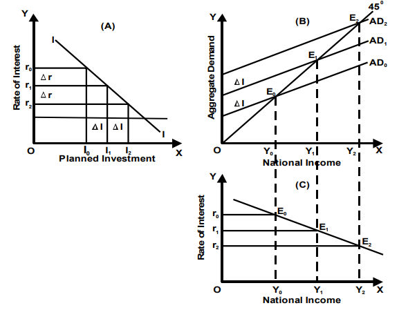
The goods market is in equilibrium when aggregate demand is equal to national income. In a closed two sector economy, the aggregate demand is determined by consumption demand and Investment demand (AD = C + I). Changes in the interest rate affect aggregate demand through changes in investment demand. With the fall in interest rates, the profitability of investment rises because the cost of investment falls. Increase in investment demand leads to increase in aggregate demand and rise in the equilibrium level of national income. The IS curve shows the different combinations of national income and interest rates at which the goods market is in equilibrium. The derivation of the IS curve is depicted in Figure given below

In panel (A) of below figure we will notice that the relationship between planned investment and rate of interest is depicted. It will be obvious from the figure that planned investment is inversely related to the rate of interest. When the interest rate falls, planned investment rises, leading to an upward shift in the aggregate demand function. The shift in the aggregate demand function is depicted in panel (B) of the figure, where in, you will see that an upward shift caused in the aggregate demand function leads to a higher level of national income in the goods market. Thus in the goods market, the level of national income is inter-connected with the interest rate through planned investment. The IS curve is the locus of various combinations of interest rates and the levels of national income at which the goods market is in equilibrium.

In panel (C) of Fig., the IS curve is depicted. It shows that the changes in the level of national income are a function of changes in the level of aggregate demand, planned investment and rate of interest. At the given rate of interest r0, the level of national income Y0 is plotted. When the interest rate falls to r1, planned investment increases to I1 and the aggregate demand function shifts from AD0 to AD1 and the goods market assumes equilibrium at Y1 level of national income. We therefore plot Y1 level of national income corresponding to r1 level of interest rate. Similarly when the interest rate further falls to r2, planned investment increases to I2 and the aggregate demand curve shifts upward to AD2. Now the goods market assumes equilibrium at Y2 level of national income. In panel (C), the equilibrium national income Y2 is shown against the rate of interest r2. By repeating this process for all possible interest rates, we can trace a series of combinations of interest rates and income levels corresponding to goods market equilibrium. By joining points such as E0, E1, E2 etc. in panel (C) of the diagram, we obtain the IS curve. You will notice that the IS curve so obtained is downward sloping indicating that when the rate of interest falls, the equilibrium national income rises.

The slope of IS curve

The IS curve has a negative slope indicating an inverse relationship between the rate of interest and the level of aggregate demand. A higher interest rate will lower the level of planned investment and hence lower the level of aggregate demand and the equilibrium level of national income. Similarly, a lower interest rate will raise the level of planned investment and hence higher will be the level of aggregate demand and the equilibrium level of national income.

The steepness of the IS curve is determined by the elasticity of investment demand curve and the size of the investment multiplier. The elasticity of investment demand shows the degree of responsiveness of investment expenditure to the changes in the rate of interest. If the investment demand is relatively elastic, a given fall in the rate of interest will result in a more than proportionate change in investment demand bringing about a larger shift in the aggregate demand curve and larger level of national income, thus making the IS curve flatter. Conversely, if the investment demand is relatively inelastic, the IS curve will be relatively steep. The steepness of the IS curve is also determined by the size of the investment multiplier. The value of the multiplier is determined by the size of the marginal propensity to consume. Greater the mpc (marginal propensity to consume), greater will be the size of the investment multiplier and greater will be the level of national income as a result of increase in investment. Thus making the IS curve flatter. Conversely, if the mpc is lower, the IS curve will have a steeper slope.

Shifts in the IS curve

Changes in autonomous expenditure causes a shift in the IS curve. Autonomous expenditure is independent of the level of income and the rate of interest. Autonomous expenditure may increase on account of increase in government expenditure, increase in autonomous consumption expenditure or increase in autonomous investment demand. Autonomous investment demand may rise due to increase in firm’s optimism about future profits. Autonomous consumption demand may rise due to households’ estimate of future incomes. Government expenditure has an autonomous component given the wide-scale use of deficit financing. An increase in autonomous expenditure at a given interest rate would shift the aggregate demand curve upwards leading to an increase in the equilibrium level of national income. With interest rate remaining constant, an upward shift in the aggregate demand curve will cause the IS curve to shift towards the right indicating increase in national income at the given interest rate.

In figure below, the shift in the IS curve is depicted by introducing the third component of the aggregate demand namely government expenditure and it is denoted by ‘G’.

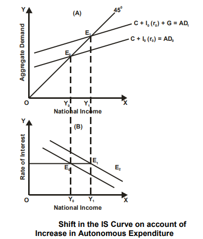
From the figure we will notice that that when the rate of interest is r0, the planned investment is I0 and the Aggregate  Demand Curve is AD which intersects the 45o line at point E0 and Y0 level of national income is determined. It is also depicted in panel (B) of the diagram by point E0. Let us now introduce the government component in the composition of the aggregate demand and assume that the entire component is autonomous in nature. Government expenditure ‘G’ will shift the aggregate demand curve to AD1 which intersects the 45 o line at point E1 higher level of national income Y1 is determined. Correspondingly, we obtain point E1 on panel (B) of the diagram as the new equilibrium point and accordingly Y1 level of national income is plotted. The change in the level of national income from Y0 to Y1 is not on account of any change in the interest rate and hence the IS curve shifts to the right. The new equilibrium point E1 is horizontally contiguous and to the right of point E0 indicating a shift in the IS curve.

The movement along the IS curve indicates shifts in equilibrium income caused by shifts in the aggregate demand curve as a result of changes in interest rates. A shift in the aggregate demand curve caused by any other factor other than interest rate must be represented by a shift in the IS curve.

The money market and the LM curve

Derivation of the LM Curve:

The LM curve is often derived from the Keynesian theory from its analysis of money market equilibrium. Consistent with Keynes, demand for money to hold depends upon transactions motive and speculative motive.

It is the money held for transactions motive which is a function of income. The greater the level of income, the greater the amount of money held for transactions motive and therefore higher the extent of cash demand curve.

The demand for money depends on the extent of income because they need to finance their expenditure, that is, their transactions of shopping for goods and services. The demand for money also depends on the speed of interest which is that the cost of holding money. This is often because by holding money rather than lending it and buying other financial assets, one has to forgo interest.

Thus demand for money (Md) is expressed as:

Md – L(Y, r)

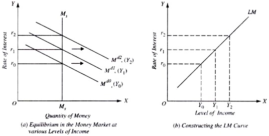
Where Md stands for demand for money, Y for real income and r for rate of interest Thus, we can draw a family of money demand curves at various levels of income. Now, the intersection of those various money demand curves like different income levels with the supply curve of money fixed by the monetary authority would gives us the LM curve.

The LM curve relates the extent of income with the rate of interest which is determined by money-market equilibrium like different levels of demand for money. The LM curve tells what the varied rates of interest are going to be (given the quantity of money and the family of demand curves for money) at different levels of income.

But the cash demand curve or what Keynes calls the liquidity preference curve alone cannot tell us what exactly the rate of interest will be. In Fig.  (a) and (b) we've derived the LM curve from a family of demand curves for money. As income increases, money demand curve shifts outward and thus the rate of interest which equates supply of money, with demand for money rises. In Fig. (b) we measure income on the X-axis and plot the income level like the various interest rates determined at those income levels through money market equilibrium by the equality of demand for and therefore the supply of money in Fig. (a).

Slope of LM Curve:

It will be noticed from Fig.  (b) that the LM curve slopes upward to the right. This is because with higher levels of income, demand curve for money (Md) is higher and consequently the money- market equilibrium, that is, the equality of the given money supply with money demand curve occurs at a better rate of interest. This implies that rate of interest varies directly with income.

It is important to understand the factors on which the slope of the LM curve depends. There are two factors on which the slope of the LM curve depends. First, the responsiveness of demand for money (i.e., liquidity preference) to the changes in income as the income increases, say from Y0 to Y1 the demand curve for money shifts from Md0 to Md1 that's , with an increase in income, demand for money would increase for being held for transactions motive, Md or L1 =f(Y).

This extra demand for money would disturb the money market equilibrium and for the equilibrium to be restored the rate of interest will rise to the extent where the given funds curve intersects the new demand curve like the higher income level.

It is worth noting that in the new equilibrium position, with the given stock of money supply, money held under the transactions motive will increase whereas the money held for speculative motive will decline.

The greater the extent to which demand for money for transactions motive increases with the rise in income, the greater the decline in the supply of money available for speculative motive and, given the demand for money for speculative motive, the higher the rise in tie rate of interest and consequently the steeper the LM curve, r = f (M2 L2) where r is that the rate of interest, M2 is the stock of money available for speculative motive and L2 is that the money demand or liquidity preference for speculative motive.

The second factor which determines the slope of the LM curve is that the elasticity or responsiveness of demand for money (i.e., liquidity preference for speculative motive) to the changes in rate of interest. The lower the elasticity of liquidity preference for speculative motive with reference to the changes in the rate of interest, the steeper is going to be the LM curve. On the opposite hand, if the elasticity of liquidity preference (money demand-function) to the changes within the rate of interest is high, the LM curve will be flatter or less steep.

Shifts within the LM Curve:

Another important thing to know about the IS-LM curve model is that what brings about shifts within the LM curve or, in other words, what determines the position of the LM curve. As seen above, a LM curve is drawn by keeping the stock or money supply fixed.

Therefore, when the money supply increases, given the money demand function, it'll lower the rate of interest at the given level of income. This is often because with income fixed, the speed of interest must fall so that demands for money for speculative and transactions motive rises to become equal to the greater money supply. This will cause the LM curve to shift outward to the right.

The other factor which causes a shift within the LM curve is the change in liquidity preference (money demand function) for a given level of income. If the liquidity preference function for a given level of income shifts upward, this, given the stock of money, will cause the rise within the rate of interest for a given level of income. This will cause a shift within the LM curve to the left.

It therefore follows from above that increase within the money demand function causes the LM curve to shift to the left. Similarly, on the contrary, if the money demand function for a given level of income declines, it'll lower the rate of interest for a given level of income and can therefore shift the LM curve to the right.

The LM Curve: The Essential Features:

From our analysis of the LM curve, we attain its following essential features:

1. The LM curve is a schedule that describes the combinations of rate of interest and level of income at which money market is in equilibrium.

2. The LM curve slopes upward to the right.

3. The LM curve is flatter if the interest elasticity of demand for money is high. On the contrary, the LM curve is steep if the interest elasticity demand for money is low.

4. The LM curve shifts to the right when the stock of money supply is increased and it shifts to the left if the stock of money supply is reduced.

5. The LM curve shifts to the left if there's an increase within the money demand function which raises the quantity of cash demanded at the given rate of interest and income level. On the opposite hand, the LM curve shifts to the proper if there's a decrease within the money demand function which lowers the amount of money demanded at given levels of rate of interest and income.

Simultaneous Equilibrium of the goods Market and Money Market:

The IS and therefore the LM curves relate the 2 variables:

(a) Income and

(b) The rate of interest.

Income and therefore the rate of interest are therefore determined together at the point of intersection of those two curves, i.e., E in Fig.  The equilibrium rate of interest thus determined is Or2 and therefore the level of income determined is OY2. At now income and the rate of interest stand in relation to each other such (1) the goods market is in equilibrium, that is, the aggregate demand equals the extent of aggregate output, and (2) the demand for money is in equilibrium with the supply of money (i.e., the desired amount of money is equal to the actual supply of money). It should be noted that LM cur/e has been drawn by keeping the supply of money fixed. Thus, the IS-LM curve model is predicated on:

(1) The investment-demand function,

(2) The consumption function,

(3) The money demand function, and

(4) The quantity of money.

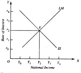
We see, therefore, that consistent with the IS-LM curve model both the real factors, namely, saving and investment, productivity of capital and propensity to consume and save, and the monetary factors, that is, the demand for money (liquidity preference) and supply of money play a part within the joint determination of the rate of interest and therefore the level of income. Any change in these factors will cause a shift in IS or LM curve and can therefore change the equilibrium levels of the rate of interest and income.

The IS-LM curve model explained above has succeeded in integrating the theory of money with the theory of income determination. And by doing so, as we shall see below, it's succeeded in synthesising the monetary and monetary policies. Further, with the IS-LM curve analysis, we are better ready to explain the effect of changes in certain important economic variables like desire to save, the supply of money, investment, demand for money on the rate of interest and level of income.

Effect of Changes in Supply of money on the rate of Interest and Income Level:

Let us first consider what will happen if the supply of money is increased by the action of the central bank. Given the liquidity preference schedule, with the increase within the supply of money, more money will be available for speculative motive at a given level of income which can cause the rate of interest to fall. As a result, the LM curve will shift to the right. With this rightward shift within the LM curve, within the new equilibrium position, rate of interest are going to be lower and therefore the level of income greater than before. This is often shown in Fig. 24.4 where with a given supply of money, LM and IS curves intersecting at point E.

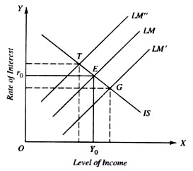
With the increase within the supply of money, LM curve shifts to the right to the position LM’, and with IS schedule remaining unchanged, new equilibrium is at point G like which rate of interest is lower and level of income greater than at E. Now, suppose that rather than increasing the supply of money, central bank of the country takes steps to reduce the supply of money.

With the reduction within the supply of money, less money will be available for speculative motive at each level of income and, as a result, the LM curve will shift to the left of E, and therefore the IS curve remaining un-changed, within the new equilibrium position (as shown by point T in Fig) the rate of interest will be higher and therefore the level of income smaller than before.

Changes in the Desire to save or Propensity to Consume:

Let us consider what happens to the rate of interest when desire to save or in other words, propensity to consume changes. When people’s desire to save falls, that is, when propensity to consume rises, the aggregate demand curve will shift upward and, therefore, level of national income will rise at each rate of interest. As a result, the IS curve will shift outward to the right. In Fig. 24.5 suppose with a particular given fall within the desire to save (or increase within the propensity to consume), the IS curve shifts rightward to the dotted position IS’. With LM curve remaining unchanged, the new equilibrium position will be established at H corresponding to which rate of interest also as level of income will be greater than at E.

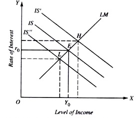
Thus, a fall within the desire to save has led to the increase in both rate of interest and level of income. On the opposite hand, if the desire to save rises, that is, if the propensity to consume falls, aggregate demand curve will shift downward which will cause the level of national income to fall for each rate of interest and as a result the IS curve will shift to the left.

With this, and LM curve remaining unchanged, the new equilibrium position will be reached to the left of E, say at point L (as shown in Fig. ) like which both rate of interest and level of national income will be smaller than at E.

Changes in Autonomous Investment and Government Expenditure:

Changes in autonomous investment and Government expenditure also will shift the IS curve. If either there's increase in autonomous private investment or Government steps up its expenditure, aggregate demand for goods will increase and this may bring about increase in national income through the multiplier process.

This will shift IS schedule to the right, and given the LM curve, the rate of interest also as the level of income will rise. On the contrary, if somehow private investment expenditure falls or the govt reduces its expenditure, the IS curve will shift to the left and, given the LM curve, both the rate of interest and therefore the level of income will fall.

Changes in Demand for Money or Liquidity Preference:

Changes in liquidity preference will bring about changes within the LM curve. If the liquidity preference or demand for money of the people rises, the LM curve will shift to the left. This is often because, greater demand for money, given the supply of money, will raise the rate of interest like each level of national income. With the leftward shift within the LM curve, given the IS curve, the equilibrium rate of interest will rise and the level of national income will fall.

On the contrary, if the demand for money or liquidity preference of the people falls, the LM curve will shift to the right. This is often because, given the supply of money, the rightward shift within the money demand curve means like each level of income there'll be lower rate of interest. With rightward shift within the LM curve, given the IS curve, the equilibrium level of rate of interest will fall and therefore the equilibrium level of national income will increase.

We thus see that changes in propensity to consume (or desire to save), autonomous investment or Government expenditure, the supply of money and therefore the demand for money will cause shifts in either IS or LM curve and can thereby bring about changes within the rate of interest also as in national income.

The integration of goods market and money market within the IS-LM curve model clearly shows that Government can influence the economic activity or the level of national income through monetary and fiscal measures.

Through adopting an appropriate monetary policy (i.e., changing the availability of money) the govt can shift the LM curve and thru pursuing an appropriate fiscal policy (expenditure and taxation policy) the govt can shift the IS curve. Thus both monetary and fiscal policies can play a useful role in regulating the extent of economic activity within the country.

Critique of the IS-LM Curve Model:

The IS-LM curve model makes a major advance in explaining the simultaneous determination of the rate of interest and therefore the level of national income. It represents a more general, inclusive and realistic approach to the determination of interest rate and level of income.

Further, the IS-LM model succeeds in integrating and synthesising fiscal with monetary policies, and theory of income determination with the theory of money. But the IS-LM curve model isn't without limitations.

Firstly, it's based on the assumption that the rate of interest is quite flexible, that is, free to vary and not rigidly fixed by the financial institution of a country. If the rate of interest is sort of inflexible, then the appropriate adjustment explained above will not take place.

Secondly, the model is additionally based upon the assumption that investment is interest-elastic, that is, investment varies with the rate of interest. If investment is interest-inelastic, then the IS-LM curve model breaks down since the required adjustments do not occur.

Thirdly, Don Patinkin and Friedman have criticised the IS-LM curve model as being too, artificial and over-simplified. In their view, division of the economy into two sectors – monetary and real – is artificial and unrealistic. According to them, monetary and real sectors are quite interwoven and act and react on one another.

Further, Patinkin has acknowledged that the IS-LM curve model has ignored the possibility of changes within the price level of commodities. According to him, the varied economic variables like supply of money, propensity to consume or save, investment and therefore the demand for money not only influence the rate of interest and the level of national income but also the prices of commodities and services.

Potemkin has suggested a more integrated and general equilibrium approach which involves the simultaneous determination of not only the rate of interest and therefore the level of income but also of the prices of commodities and services.

Key takeaways - The IS-LM model shows how the equilibrium levels of income and interest rates are simultaneously determined by the simultaneous equilibrium in the two interdependent goods and money markets.

3.2 Inflation and unemployment : Philips curve

In 1958, AW Phillips, a professor at the London School of Economics published a study of wage behavior in the United Kingdom for the years 1861 and 1957. Phillips found an inverse relationship between the rate of unemployment and the rate of inflation or the rate of increase in money wages. The higher the rate of unemployment, the lower the rate of wage inflation i.e. there is a tradeoff between wage inflation and unemployment. The Phillips curve shows that the rate of wage inflation decreases with the increase unemployment rate. Assuming Wt as the wages in the current time period and Wt+1 in the next time period, the rate of wage inflation, gw, is defined as follows:

By representing the natural rate of unemployment with u* , the Phillips curve equation can be written as follows:

Where ε measures the responsiveness of wages to unemployment. This equation states that wages are falling when the unemployment rate exceeds the natural rate i.e. when u > u* , and rising when unemployment is below the natural rate. The difference between unemployment and the natural rate, u – u * is called the unemployment gap. Let us assume that the economy is in equilibrium with stable prices and the level of unemployment is at the natural rate. At this point, if the money supply increases by ten per cent, the wages and the price level must rise by ten per cent to enable the economy to be in equilibrium. However, the Phillips curve shows that for wages to rise by ten per cent, the unemployment rate will have to fall. A fall in the unemployment rate below the natural level will lead to increase in wage rates and prices and the economy will ultimately return to the full employment level of output and unemployment. This situation can be algebraically stated by rewriting equation one above as follows.

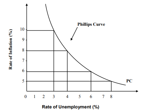
Thus for wages to rise above their previous level, unemployment must fall below the natural rate. The Phillips curve relates the rate of increase of wages or wage inflation to unemployment as denoted by equation two above, the term ‘Phillips curve’ over a period of time came to be used to describe a curve relating the rate of inflation to the unemployment rate. Such a Phillips curve is depicted in Fig.

Its observed that when the rate of inflation is ten per cent, the unemployment rate is three per cent and when the rate of inflation is five per cent, the rate of unemployment increases to eight per cent. Empirical or objective data collected from other developed countries also proved the existence of Phillips Curve. Economists believed that there existed a stable Philips Curve depicting a tradeoff between unemployment and inflation. This trade-off presented a dilemma to policy makers. The dilemma was a choice between two evils, namely: unemployment and inflation. In a dilemma, you chose a lesser evil and inflation is definitely a lesser evil for policy makers. A little more inflation can always be traded off for a little more employment. However, further empirical data obtained in the 70s and early 80s proved the non-existence of Phillips Curve. During this period, both Britain and the USA experienced simultaneous existence of high inflation and high unemployment. While prices rose rapidly, the economy contracted along with more and more unemployment.

Keynesian explanation of Philips curve

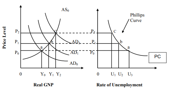
The explanation of Phillips curve by the Keynesian economists is shown in the below Fig. Keynesian economists assume the upward sloping aggregate supply curve. The AS curve slopes upwardly due to two reasons. Firstly, as output is increased in the economy, the law of diminishing marginal returns begins to operate and the marginal physical product of labor (MPPL) begins to decline. Since the money wages are fixed, a fall in the MPPL leads to a rise in the marginal cost of production because MC = W/ MPPL. Secondly, the marginal cost goes up due a rise in the wage rate as employment and output are increased. Following rise in aggregate demand, demand for labor increases and hence the wage rate also increases. As more and more labor is employed, the wage rate continues to rise and the marginal cost of firms increases. You may notice that in Panel (a) of  the below fig that with the initial aggregate demand curve AD0 and the given aggregate supply curve AS0, the price level P0 and output level Y0 are determined. When the aggregate demand increases, the AD0 curve shifts to the right and the new aggregate demand curve AD1 intersects the aggregate supply curve at point ‘b’. Accordingly, a higher price level P1 is determined along with a rise in GNP to Y1 level. With the increase in the real GNP, the rate of unemployment falls to U2. Thus the rise in the price level or the inflation rate from P0 to P1, the unemployment rate falls down thereby depicting an inverse relationship between the price level and the unemployment rate. Now when the aggregate demand further increases, the AD curve shifts to the right to become AD2. The new aggregate demand curve AD2 intersects the aggregate supply curve at point ‘c’. Accordingly, the price level P2 and output level Y2 is determined. The level of unemployment now falls to U3. In Panel (b) of the figure, points a, b and c are plotted and these points corresponds to the three equilibrium points a, b and c in Panel (a) of the figure. Thus a higher rate of increase in aggregate demand and a higher rate of rise in price level are related with the lower rate of unemployment and vice versa. The Keynesian economists were thus able to explain the downward sloping Philips curve showing inverse relation between rates of inflation and unemployment.

Key takeaways –

3.3 Stagflation : meaning, causes, and consequences

Stagflation refers to a situation when a high rate of inflation occurs simul­taneously with a high rate of unemployment. The existence of a high rate of unemployment means the reduced level of GNP.

The term stagflation was coined during seventies when several developed countries of the world, received a supply stock in terms of rapid hike in oil prices. In 1973, the Cartel of Oil Producing Countries OPEC raised the worth of oil.

There was a fourfold increase in the oil prices. In the us during 1973-75 the higher costs of fuel-oil and other petroleum products caused a sharp increase in the prices of manufactured goods. The rate of inflation went up to over 12 per cent during 1974 in USA.

A severe recession, the worst since 1930s, also hit the Ameri­can economy during the 1973-75. The real GNP declined between the late 1973 and early 1975. As a consequence, the rate of unemployment shot up to just about 9 per cent.

Thus, both inflation and unemployment were unusually very high during this era (1973-75). This simultaneous oc­currence of high inflation and high unemployment was also seen just in case of other free market devel­oped countries like Britain, France and Germany. The recovery from recession began in 1975 and over subsequent few years GNP rose and unemployment declined. Rate of inflation also declined from over 12 per cent to the range of 5 to 7 per cent.

But, again in 1979 when a revolution in Iran created a crises in world oil market, OPEC doubled the worth of oil. This brought back stagflation again in 1979 within the developed countries. Real gross national product fell at a rapid rate during 1979-81. Rate of inflation again went up to over 10 per cent in these countries during this era .

India also couldn't shake the oil price shocks in 1973 and 1979. But, just in case of India, oil price triggered cost-push inflation but didn't give rise to stagflation as the term is usually inter­preted in 1973 and 1979. The general public investment in India picked up from 1974 which generated economic growth.

Definition

Stagflation is an unusual economic situation in which high inflation (leading to increasing prices) coincides with increasing unemployment rates and decreasing levels of output/stagnation of economic growth. That’s why it’s called “stagflation”: it’s a clear combination of inflation and economic stagnation. Economic stagnation is defined as an extended span of minimal or nonexistent economic growth (generally, that means under 2 or 3 percent growth annually).

Causes of Stagflation:

Stagflation has a number of potential causes, including:

Different explanations of stagflation are given by eminent economists. It's worth noting that causes of stagflation in India during 1991-94 are different from those given by the economists for stagflation of 1973-75 and 1979-81 within the developed capitalist economies like those of USA, Great Britain. We'll first explain stagflation in USA, Great Britain and other developed capitalist countries during 1973-1975 and again in 1979-81 so dwell on stagflation in India.

Adverse Supply Shocks:

The main reason why typical stagflation arose within the developed capitalist economies during seventies and early eighties was the adverse supply shocks that oc­curred during these two periods. As mentioned above, there was fourfold increase in oil prices by OPEC following Arab-Israel war in 1973 then again doubling of oil prices by it in 1979 following the Iranian Revolution which pushed up the energy costs of the economies and re­sulted in higher product prices.

In terms of aggregate supply curve, this cost-push factor de­livered by oil price shock is interpreted as a de­crease or leftward shift within the aggregate supply curve. How this adverse supply shock caused stagflation within the developed capitalist world is illustrated in the below fig where initially aggregate demand curve AD0 and aggregate supply curve AS0 intersects at E0 and determines the price level adequate to P0.Stagflation Arising from an Adverse Supply Shock

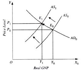
Since adverse supply shock delivered by hike in oil prices raises the value per unit of production, aggregate supply curve shifts upward to the left to the new position AS1. With the aggregate demand curve AD0 remaining unchanged, the new aggregate supply curve AS1 intersects it at E1. It'll be seen that within the new equilibrium position price level rises to P1 and GNP falls to Y1. Thus, adverse supply shock causes cost-puch inflation along side a reduction in the level of GNP.

A reduction in GNP implies a rise in unemployment rate and occur­rence of recession. Thus, an adverse sup­ply shock causes both high inflation and high unemployment rate. It's going to be noted that so as to urge out of recession and to reduce unemployment, if Government seeks to lift aggregate demand to the higher level AD1 by adopting expansion­ary fiscal and monetary policies, the new equilibrium is reached at point E2 (see below fig) and as a result price index rises to P2, while the real GNP comes back to the first higher level Y0 where financial condition of labour prevails.

Further Surge in rate of inflation If Aggregate Demand is Raised to urge Out of Stagflation

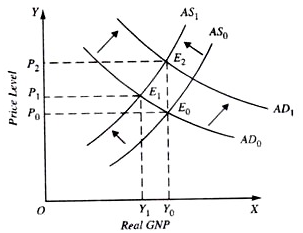
Thus during this context of stagflation in the economy attempts by the government to raise aggre­gate demand to urge out of recession and reduce unemployment end in further rise within the rate of inflation . This shows that mere management of demand is sort of inappropriate to solve the problem of stagflation.

Though rise in oil prices has been a chief supply shock received by all the economies of the world which imported oil from Middle East Countries causing stagflation of 1970s and early 1980s, there also are other sorts of adverse supply shocks which occur.

In different countries differ­ent types of supply shocks may occur bringing about rise in unit cost of production and causing a leftward shift within the aggregate supply curve. This has caused stagflation episodes from time to time. Just in case of USA, besides oil price shocks, the opposite supply shocks explained below also contributed to the stagflation of 1973-75.

An important supply shock operating in the USA was the shortage in supplies of agricultural products during this era . This happened because a good amount of american agricultural prod­ucts had to be exported to Asia and therefore the soviet union where severe shortfall in production occurred in 1972 and 1973.

Larger exports reduced the domestic supplies of agricultural products used as staple within the production of industries producing food and fibre products. This raised the cost of production of those commodities and their higher costs were passed on to the consumers as higher prices. This resulted in shifting of the mixture supply curve to the left.

It is important to notice that the upper prices of agricultural commodities like sugar cane, cotton, food-grains which can occur because of either shortfall in production or because of the rise in their procurement prices has often been working also in the Indian economy which has resulted in higher costs to the industries pro­cessing these agricultural products.

Another adverse supply shock that occurred within the USA during the amount of 1971-73 causing stagflation episode of 1973-75 was depreciation of dollar. Depreciation of dollar means price of dollar in terms of foreign currencies was reduced.

This raised the prices of american imports. To the extent the imports were used as inputs in American industries, unit production costs went up causing a shift within the aggregate supply curve to the left. Within the period of 1973-75, removal of wage and price controls which had been imposed earlier also produced a supply stock to the American economy.

As these wages and price controls were lifted, workers got their wages increased and business firms pushed up the prices of their products. This also contributed to stagflation of 1973-75 in the USA.

Inflationary Expectations:

Besides supply shocks explained above, another important cause of stagflation of seventies was inflationary expectations which were prevailing at that time. These inflationary expectations at that point in the USA were caused by greatly increased military expendi­ture incurred on the Vietnam War in the late 1960s.

In the early seventies workers with expectations of inflation to continue pressed for higher wages to catch up on accelerating inflation. Business firms within the context of mounting inflation didn't resist labour demand for higher nominal wages. They granted the higher wages which raised unit cost of production and resulted in shifting of aggre­gate supply curve to the left. This also contributed to bringing stagflation.

End of Stagflation in the USA: 1982-88:

As explained above, there have been two bouts of stagflation in the several countries of the world, first during the amount 1973-75 and, second, during the period 1979-81. However, during 1982-88 thanks to favourable supply shocks and occurrence of other favourable factors, stagflation of the earlier period came to end. The important favourable supply shocks were the decline in oil prices by OPEC during this period. This caused the mixture supply curve to shift to the right bringing about fall in both inflation and unemployment.

Another important factor contributing to the demise of stagflation in 1982-88 in USA was the deep recession that overtook the American economy in 1981-82 which was mainly caused by tight monetary policy pursued by Federal Bank.

Such was the severity of recession that unemployment in USA rose to 9.7 per cent in 1982. Due to this high percentage workers accepted smaller increases in their nominal wages or in some cases accepted even reduction in their wages.

Further, due to still foreign competition and their eagerness to maintain relative shares in domestic and for­eign markets, business firms were restrained to boost prices of their products. This also worked to bring stagflation to finish .

It is important to note that while during the periods of stagflation in 1970s and early 1980s, both inflation and unemployment simultaneously increased, during the expansion period of 1982-88 when stagflation nearly subsided both inflation and unemployment rates fell simultaneously.

Key takeaways –

3.4 Supply side economics

Supply-side economics is a relatively new term which came into use in the mid-1970s as results of the failure of Keynesian demand-side policies within the US economy which led to stagflation. The term is new but its basic principles are to be found within the works of the classical economists. According to J.B. Say, supply creates its own demand.

The very act of supplying goods implies a demand for them. If there's an imbalance between demand and supply, it's corrected automatically by changes in prices and wages and therefore the economy always tends toward full employment.

The main emphasis of the classical economists was on economic growth for which they advocated non-interference with the market mechanism. It had been the “invisible hand” which led to the maximisation of national wealth.

They believed that entrepreneurs, investors and producers were the prime movers on which the economy depended. It was the increase within the supplies of capital and labour and increase in their productivities that determined growth. Of course, trade and capital movements internationally were instrumental in a faster growth rate of the economy.

Main Features of Supply-Side Economics:

Modern supply-side economics lays emphasis on providing all kinds of economic incentives to raise aggregate supply within the economy. According to Bethell, “The essential argument of supply-side theory is that adding to supply unlike adding to demand isn't a zero-sum task. In order to make something,… a producer does not need to tend any money. Instead, he has got to tend an incentive.” Incentives to producers are essential to invest, produce and employ. Similar incentives are to be given to individuals to work and save more.

The government plays a limited role in liberalising markets, reducing taxes and freeing the labour market. The main objectives of supply-side policies are to keep inflation at a low level, achieve and maintain full employment and attain faster economic growth. Supply-side economists suggest the subsequent policy measures in order to attain these objectives.

Tax-induced Change in Aggregate Supply:

Supply-siders regard tax cuts as an effective means of raising the growth rate of the economy. To assess the likely effects of tax reductions, they distinguish between income and substitution effects of a cut within the marginal rate of tax.

The substitution effect of a wage cut induces people to work more and have less leisure, and therefore the income effect causes people to work less and enjoy more leisure. It’s only when the substitution effect of a tax cut is larger than the income effect that there'll be an incentive to figure more, thereby resulting in reduction in unemployment.

A reduction in personal tax rates increases the incentive of people to work and save more. High savings reduce short-term interest rates and lead to increased investment and thus to an increase within the economy’s capital stock. Reduction in marginal tax rates by improving the work effort of the people also increases their productive capacity and therefore the level of output and employment within the economy.

Thus supply-side tax cuts by raising work, effort, saving and investment, increase the supplies of labour and capital and shift the aggregate supply curve to the right. The effect of a. Supply-side tax cut is illustrated in the below Fig. Where AS is that the aggregate supply curve and AD is that the given demand curve.

Real output or GDP is measured along the horizontal axis and the price level on the vertical axis. AS and AD curves intersect at point T and determine OP price and OQ real output of the economy. Suppose there's a tax cut both on persons and firms. This increases work effort and saving on the part of workers and investment by firms.

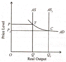
As a result, supplies of labour and capital increase which shift the aggregate supply curve on the right as AS1. Now the AS1 curve cuts the AD curve at point C. As a result, the price level falls to OP1 and the real output increases to QQ1 as a results of a tax cut.

Similarly, reduction in corporate tax rates, by giving incentives to the corporate sector in the sort of increasing tax credit for larger investment and providing higher depreciation allowance, encourage investment. Higher investment results in the production of more goods and services per unit of labour and capital.

Supply-siders also advocate an extra tax relief for firms employing researchers because R&D helps in increasing productivity. They also favour reduced estate taxes for small farmers which will induce them to spend more on inputs so as to increase production.

Further, tax cuts reduce diversions to “shelter” (protected) industries and minimise or eliminate the necessity for accountants, investment consultants and tax-lawyers. Moreover, tax reductions reduce ‘underground’ (black market) activity where exchange isn't recorded within the books and no taxes are paid.

Increasing Growth Rate:

According to supply-side economists, tax cuts increase the disposable income of the people who raise additional demand for goods and services. On the opposite hand, the faster growth in productivity results in the assembly of additional goods and services to match the additional demand.

This leads to balanced growth in the economy without shortages. When the economy is moving towards balanced growth, the rate of inflation is low. This, in turn, results in an increase within the real disposable income of the people which raises consumption, output and employment.

Low inflation results in increase in net exports which strengthen the value of national currency in relation to foreign currencies. The increase in productivity increases the production of more goods for export, thereby further strengthening the country’s currency.

Thus supply-side economists advocate reduction -in tax rates in order to increase the incentives to work, save and invest and to get more tax revenue by the govt. Increase in investment leads to an increase within the economy’s capital stock, to increase in productivity, to larger output, low inflation, high level of employment and high rate of growth of the economy.

These policy prescriptions shift the aggregate supply curve of the economy to the right. This is illustrated in the below Fig where AS is that the aggregate supply curve and AD is that the given aggregate demand curve. They intersect at point E which is that the initial equilibrium point of the economy with OP price level and OQ real output.

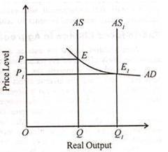
Suppose the supply-side policies increase the total supply of factors like labour and capital because of tax policies, incentives, etc. They increase real output and shift the AS curve to the right as AS1. The new equilibrium is at where the AS1 curve cuts the AD curve. Now real output increases to OQ1 and the price level falls to OP1 thereby increasing the growth rate of the economy.

Keynesian economics

Keynesian economics was born during the great depression of the 1930s, when an outsized percentage of labour force (about 25%) was rendered unemployed and also a good deal of productive capacity (i.e., capital stock) lay idle leading to an enormous decline in Gross National Product (GNP) of the economies.

The prices were actually falling during this depression period. When after the Second war, problem of inflation instead of unemployment became the main concern of the economists. Keynesian economists explained it in terms of excess aggregate demand and thus called it demand-pull inflation.

Keynes and his followers laid emphasis on the management of aggregate demand to cause short-run stability within the economy. They recommended expansionary fiscal and monetary policies to boost aggregate demand to pull the economy out of depression or recession and thereby to reduce unemployment. On the opposite hand, to fight inflation, they advocated contractionary fiscal and monetary policies to reduce aggregate demand.

However, the matter of stagflation encountered in the USA and Great Britain during the seventies and early eighties when both high inflation and high unemployment prevailed simultaneously didn't admit of easy solution through the Keynesian demand management policies. In fact, attempts to remedy the stagflation through Keynesian demand management worsened things.

Against this backdrop an alternative school of considered macroeconomics was put forward. This alternative thought laid stress on supply-side of macroeconomic equilibrium, that is, it focused on shifting the mixture supply curve to the right rather than causing a shift in aggregate demand curve.

Thus, economics prefers to solve the problem of stagflation, that is, simultaneous existence of high inflation and high unemployment through management of aggregate supply rather than management of aggregate demand.

Further, supply-side economics stresses the determinants of long-run growth rather than causes of short-run cyclical changes within the economy. Supply-side economists lay emphasis on the factors that determine the incentives to figure, save and invest which ultimately determine the aggregate supply of output of the economy.

Difference in the approaches of Keynesian demand-side theory and alternative supply-side theory are often understood with regard to below Fig which illustrates the emergence of stagflation as a consequence of a shift within the aggregate supply curve thanks to the cost-push factors and decline in productivity.

Suppose aggregate supply curve shifts upward to the left from AS1 to AS0 due to some cost-push factors (e.g., rise in oil price). As a result, it'll be seen from Figure that price level would rise to P1 and output (i.e., real GNP) would fall to Y1 (which will cause increase in unemployment).

This high inflation and high unemployment configuration represents the state of stagflation. Now, the supply-side economists argue that to get out of stagflation, aggregate supply curve should be shifted to the right. As is clear from the Fig. 26.3 with the rightward shift of the aggregate supply curve from AS1 to AS0, the economy moves from the equilibrium point E1 to point E0 showing that while price index falls, aggregate national output increases (which will reduce unemployment). Thus, during this way, through management of aggregate supply, the economy are often lifted out of stagflation.

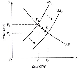
It's worth mentioning that if to tackle this problem of stagflation Keynesian policy of increasing aggregate demand, that is, shifting the aggregate demand curve from AD0 to AD1 (see Fig.) through expansionary fiscal and monetary measures is adopted to reduce unemployment, it'll cause price index to rise further to P2 and can thus worsen the inflationary situation.

On the opposite hand, if to tackle inflation, aggregate demand is reduced to AD0, though i will cause the price level to fall, it'll end in reduction in real aggregate output (GNP) causing unemployment to increase further and thus deepen the recession.

Therefore, supply-side economists contend that Keynesian demand-management policy fails to supply an answer for the problem of stagflation. The supply- side economists, the prominent among whom is Laffer , are of the view that policy , especially of taxation, are often used to stimulate incentive to work, save and invest and task risks which cause increases in aggregate supply and yield higher growth in productivity. This results in higher growth of real gross national product and lower both rates of inflation and unemployment.

Basic Propositions of Supply-side Economics:

1. Taxation and Labour-Supply:

The first important basic proposition of supply-side economics is that cut in marginal tax rates will increase labour supply or work effort as it will raise the after-tax reward of labour. The increase in labour supply will cause growth in aggregate supply of output. According to them, beyond some point a higher marginal tax rate reduces people’s willingness to work and hence reduces labour supply in the market.

They argue that how long individual will work depends upon how much the additional after tax income (i.e., after-tax wage rate) will be earned from the extra work-effort made. Lower marginal tax rates by increasing after tax earnings of extra labour would induce people to work longer hours. The increase in after-tax earnings as a result of reduction in marginal tax rate raises the opportunity cost of leisure and provide incentives to the individuals to substitute work for leisure. As a result, aggregate labour supply increases. Further, by ensuring higher reward from work, lower marginal tax rates encourage more people to enter the labour force.

This also increases the aggregate labour supply in the market. Thus, increase in labour supply following the reduction in marginal tax rates can occur in several ways by increasing the number of hours worked per day or per week, by inducing more people to enter the labour force, by providing incentives to workers to postpone the time of retirement, and by discouraging workers from remaining unemployed for a long period.

Reduction in marginal tax rates on business income raises the after-tax return on labour em­ployed. This will encourage businesses to demand and employ more labour. Thus reduction in mar­ginal tax rates on incomes will increase both the supply of labour and demand for it.

2.  Incentives to Save and Invest:

The second basic proposition of supply-side economics is that reduction in marginal tax rates will increase the incentives to save and invest more. According to it, a high marginal tax rate on incomes reduces the after-tax return on saving and investment and therefore discourages saving and investment. Suppose an individual saves Rs. 1000 at 10 per cent rate of interest, he will earn Rs. 100 as interest income per annum. If marginal tax rate is 60 per cent, his after-tax interest income will be Rs. 40. This means that after-tax interest on his savings has fallen to 4 per cent (40/1000 × 100 = 4).

Thus, whereas an individual might be willing to save at 10 per cent rate of return on his saving, he might prefer to consume more rather than save when the return he gets is only 4 per cent. To promote savings, it may be noted, is essential for raising investment and capital accumulation which in the long run determines growth of output.

The supply-side economists emphasise lower marginal tax rates on income to encourage savings. They also argue for lower tax rates especially on income from investment such as business profits to induce businessmen and firms to invest more. It will be recalled that investment in an economy depends to a great extent on expected rate of profits (or what is called marginal efficiency of investment).

A higher tax on business profits and corporate income discourages investment by reducing the after-tax net profit on investment. Thus, lower marginal tax rates on business profits will encourage saving and investment and step up capital accumulation. With more capital per worker, labour productivity will rise which will tend to reduce unit labour cost and lower the rate of inflation.

Moreover, the higher rate of capital accumulation, will ensure greater growth of productive capacity. The lower unit labour cost and the higher rate of capital accumulation made possible by greater saving and investment will cause aggregate supply curve to shift to the right. This will lower the price level, increase the growth of output and reduce unemployment.

3. Cost-Push Effect of the Tax Wedge:

Another important proposition of supply-side econom­ics is that the substantial growth of public sector in the modern economies has necessitated a large increase in the tax revenue to finance its activities. The tax revenue has increased both absolutely and as a percentage of national income. The Keynesian economists view the tax revenue as with­drawal of money income from the people which operates to reduce aggregate demand.

Thus, in the Keynesian view the mobilisation of resources for the public sector through taxation has an anti- inflationary effect. On the contrary, supply-side economists think that sooner or later most of the taxes, especially excise duties and sales taxes, are incorporated in the business costs and shifted to the consumers in the form of higher prices of products.

Thus, in their view, imposition of higher taxes, like higher wages, have a cost-push effect. Referring to the period of seventies and early eighties in the USA, which was plagued by the great stagflation, they point out that huge increases made in sales and excise taxes by the state and local Governments and substantial hike in payroll taxes by Fed Government in the USA during this period had greatly pushed up the business costs resulting in higher product prices.

In fact, supply sides contend that many taxes constitute a wedge between the costs incurred on resources and the price of a product. With the substantial growth of the public sector, the funds required to finance it have greatly increased resulting in a greater tax wedge. This has worked to shift the aggregate supply curve to the left.

4. Underground Economy:

Another important contention of supply-siders is that higher mar­ginal tax rates encourage people to work in the underground economy (which in India is popularly called black or parallel economy) where their income cannot be traced by the income tax depart­ment.

In India, this underground economy is very large. Not only individual businessmen evade income taxes, corporate firms also have devised several illegal ways to evade taxes on their profits. It is not only taxes on personal income and company profits but also excise duties and sales taxes which are not paid fully by individuals and companies.

In line with the supply-side view, the former Finance Minister Dr. Manmohan Singh has often argued in favour of reduction in taxes. According to him, lower tax rates would increase tax compliance which increases the amount of income which people will report to the taxation authorities. Thus, the supply-side economists think that reduction in taxes will in fact raise the tax revenue by discouraging people from evading taxes and from operating in the underground economy.

5.  The Laffer curve: tax rate Vs. Tax Revenue:

The most popular aspect of supply-side economics is the Laffer curve named after its originator Prof. Laffer. The Laffer curve depicts the relation between tax rate and tax revenue. It’s based on the assumption that a cut in the marginal rate of tax will increase the incentives to work, save and invest. This tax cut, in turn, will increase the tax revenue. The Laffer curve shows two extremes of rate s: A 0% tax rate and a 100% tax rate.

Both yield no tax revenue. If the tax rate is 0%, no revenue will be raised. If the tax rate is 100%, people will have no incentive to work, save and invest in the least because the entire income will attend the govt. Thus the tax income will again be zero. As the tax rate increases from 0% to 100%, tax revenue correspondingly rises from zero to some maximum level then starts declining to zero. Thus the optimum tax rate is somewhere between the two extremes.

Figure shows the Laffer curve where the tax rate (0%) is taken on the horizontal axis and therefore the tax income on the vertical axis. As the tax rate is raised above zero, the tax revenue starts increasing. The Laffer curve is upward sloping. At the relatively low rate, it's upward sloping. At the relatively low tax rate T1, the tax revenue is R1.

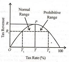
As the rate rises to T, the tax income continues to increase and the curve reaches the peak, P where the tax revenue R is the maximum. Thereafter, further rise in the tax rate will reduce revenue to the govt. Thus T is the optimum rate of tax.

According to Laffer, “Except for the optimum rate, there are always two tax rates that yield the same revenue.” within the figure, the revenue R1 at the high tax rate T2 is the same as the revenue collected at the low rate T1. If the govt wishes to maximise tax revenue, it'll choose the optimum tax rate T.

An important feature of the Laffer curve is that it's a normal range and a prohibitive range. The normal range is to the left of the optimum rate T and the prohibitive range is to its right. Within the normal range, increases within the tax rate bring more revenue to the govt.

But within the prohibitive range, when the rate becomes high, it reduces the incentives to work, save and invest. Consequently, the fall in output more than offsets the rise in rate. When the rate reaches 100%, the revenue falls to zero because no one will bother to work.

Thus high rate stifles economic growth and results in high unemployment. Therefore, a reduction in the tax rate will actually increase revenue by encouraging the incentives to work, save and invest. People not only produce and earn more but also switch money out of low-yielding “tax shelters” and untaxed “underground” economy into more productive and socially desirable investment. The result would be higher employment and economic growth leading to high tax revenue.

Criticisms of Supply-side Economics:

The above prescriptions of economics are criticised by economists on the subsequent grounds:

1. Laffer curve Controversial:

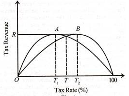
The Laffer curve is an interesting but a controversial concept. Nobody knows with certainty either the location of the optimum point or the exact shape of this curve. The curve may peak at 40% or 90% tax rate, or it may peak in-between these rates.

For instance, if we take the curve which peaks at point A in the below Figure, the present tax rate-T should be move T1 to maximise revenue. On the opposite hand, if another curve peaks at point B, the rate T should be increased to T2. Without the knowledge of either the peak or the shape of the curve, it's not possible to know the effect of reducing (or increasing) the tax rate or tax revenue and economic activity. In fact, nobody knows the exact shape of the Laffer curve or the relationship between tax rate and tax revenue.

2. Tax Cuts do not bring High Growth Rate:

Economists don't agree that cutting tax rates will lead to high rate of growth and more tax revenue. They mean that high growth rate generates higher incomes which, in turn, generate higher tax revenue. Therefore, it's not reduction in tax rates that leads to the high growth rate of the economy.

3. Tax Cuts do not measure Work Effort:

It is not possible to measure work effort specifically as results of tax cut. No doubt, increased work effort leads to higher incomes and to increase in tax revenue. But the increased tax revenue might not be sufficient to compensate the govt for the decrease in revenue because of the lower tax rate. Moreover, it's possible that people may work less when their disposable income increases with the lower tax rate.

4. Tax Cuts don't affect Target Incomes:

Critics argue that some persons have ‘target’ real income. When taxes are reduced, they're going to work less and have more leisure to maintain their target income.

5. State Intervention Necessary:

Supply-siders are criticised for their policy of non-intervention by the state. But there are many contradictions within the working of the capitalist system which cannot sustain balanced growth of the economy. When the economy reaches full employment, variety of distortions and imbalances develop which fail to maintain full employment. Therefore, state intervention is important to remove them.

6. Supply-side Policies fail to bring Social Justice:

Supply-side economists emphasise reduction in social spending, subsidies, grants and budget deficit with reduction in taxes. But such a policy has actually led to large budget deficits in the United States. Further, the policy of reducing social spending, subsidies and grants adversely affects the poor and unemployed and fails to bring social justice.

Key takeaways –

Case study

India’s Agricultural Sector Slipping into Stagflation

Indian governments hate inflation , but inflation seems attached to this government like an irritating limpet. For most of 2010, the government battled to bring down the rate at which prices went up and by November, 2010 its efforts seemed to be working: headline inflation slipped to 7.5%. But the following month, it’s roared back up to 8.4%. Worse, the surge is being driven by something that hits people straight in the gut: food prices.

This worried everyone, including Prime Minister Manmohan Singh so much, that he spent two days last week meeting his senior Cabinet colleagues to find out exactly what’s driving prices up and what to do about it.

Most of the time, prices go up because there’s too much money chasing too few things. Notes That sort of inflation is relatively easy to bring to heel, by getting central banks to raise interest rates and suck out the excess cash from the system. That, alas, doesn’t seem to be working anymore.

News

Sources-