Unit I

Introduction to Operations Research and Linear Programming

1.1 Introduction to Operations Research

• Operations Research - Definition, Characteristics of OR, OR Techniques, Areas of Application, Limitations of OR.

Meaning and definition of operations research:

This is an analytical method that helps management make decisions. The name of this method is that research (O.R.) is comparatively new, but the tactic used for it's not new. Operations research involves the application of scientific principles and methods to strategic issues.

The subject of operations research was born in the United Kingdom during World War II and was used in military strategy. During World War II, a group of scientists with representatives from mathematics, statistics, physics, and social sciences was commissioned to study various military operations. The team was very successful and contributed significantly to the meticulous response to the overall operation and related operational issues.

As military strategies and their decisions were so important and costly that it became necessary to allocate such research to operations, the best scientists were grouped with the support of military institutions to develop scientific methods and methods. Adopted and provided quantitative information Decision.

After World War II, its application began in industry, trade, agriculture, planning and various other economic areas.

Operations research can be defined as:

Definition:

(I)       Application of scientific methods, techniques, and tools to problems related to operating the system in order to provide system controllers with the best solution to the problem.

(II)    Research may be a tool for creating decisions that seek optimal results that are like the general purpose and constraints of the organization.

(III)  O.R. Is a scientific method that provides the executive department with a quantitative basis for making decisions about the operations under its control?

(IV)  A scientific approach to problem solving for management.

(V)   It helps executives make decisions by providing the necessary quantitative information based on scientific analysis.

(VI) It is the requisition of the latest methods of mathematical science to complicated problems involving the management of huge systems of labor, machinery, materials, and money in industry, business, government, and defence. A distinctive approach is to develop a scientific model of the system that comes with measurement of things like chance and risk to predict and compare the result of alternative decisions, strategies, or controls.

(VII) It is the application of scientists and subject experts to the study of specific manipulations of the scientific method. Its purpose is to provide management, which is the basis for quantitatively predicting the most effective outcomes of operations under a given set of variable conditions, thereby providing a sound basis for "decision-making". That is.

In fact, operations research uses research and scientific methods for analysis, as well as for investigating current and future problems. Therefore, operations research provides management with an alternative plan for the problem to make a decision.

It is very clear that Operations Research does not make management decisions, but instead, this method presents management with a careful scientific and quantitative analysis of the problem, allowing management to make healthier decisions. You will be during a better position to try to.

It can be used to solve various types of problems, including:

1. Problems with queues, unit arrivals, or those in need of service.
2. Issues related to the distribution of materials and activities among limited facilities.
3. Equipment replacement problem.
4. Problems related to production processing, that is, production control and material shipment.

However, you may remember that operations research never replaces managers as decision makers. The ultimate and complete responsibility for analysing all factors and making decisions rests with the manager.

In a broader sense, operations research does not deal with everyday issues such as output or machine capacity by a single worker. Instead, it concerns the overall aspects of business operations, such as inventory, sales, production, and scheduling relationships. It may also trades in with the overall circulation of goods and services from the factory to the consumer.

The operations research team may include statisticians, psychologists, labor professionals, mathematicians, etc., depending on the requirements of the problem.

Operations Research Phase:

Since then, the main purpose of operations research has been to provide better quantitative information for decision making. Now our goal is to learn how to make better decisions.

The decision-making process in OR research typically involves the following phases:

1. Judgment stage:

1. Operation decision.
2. Determining the purpose.
3.  Judgment of the effectiveness of measures.
4.          Identify the type of problem, its cause, and the cause.

B.    Survey phase:

1. Observation and data collection to better understand the problem
2. Formulation of relevant hypotheses and models.
3. Analysis of available information and verification of hypotheses.
4.  Generate and generate results, and consider alternatives.

C.   Action phase:

1. Recommendations for corrective action for those who first raised the issue. This includes assumptions made, scope and limits, alternative course of action and its effects.
2.  Make the solution work: Implementation.

In the absence of an OR, these phases are often performed completely, otherwise important steps are skipped. Judgment and subjective decision making are not enough. Therefore, the industry is looking for more objective ways to make decisions from operations research. It turns out that the method used also needs to take into account emotional and subjective factors.

For example, skills and a creative workforce are key elements of our business, and if a manager wants to have a new place, he considers the employee's personal feelings about the place he chooses is needed.

Scope of operations research:

In recent organized development, O.R we have successfully resolved many research cases in the military, government, and industry. The basic problem of most developing countries in Asia and Africa is to get rid of poverty and hunger as soon as possible. Therefore, economists, statisticians, managers, politicians, engineers work in teams, O.R. There is a large range to solve this problem approach.

On the other hand, due to the rapid population growth and the accompanying food shortages, countries face the problem of optimally allocating land to different crops, depending on climatic conditions and available facilities. Developing countries face the problem of optimal distribution of water from resources such as canals for irrigation purposes. Therefore, a considerable amount of scientific research can be done in this direction.

In the field of industrial engineering, there are problems from procuring materials to shipping finished products. Management is always interested in optimizing profits.

Therefore, to make a scientifically based decision, O.R the research team will consider various alternatives and their impact on existing systems. This approach is equally useful for economists, managers, planners, irrigation or agriculture professionals and statisticians.

The operations research approach is useful for operations management. Operations management can be defined as the management of a system for providing goods or services and involves the design and operation of the system for manufacturing, transportation, supply, or service. The operating system translates the input to meet the needs of the customer.

Therefore, operational management is concerned with optimal resource utilization, that is, effective use of resources with minimal loss in utilization or waste. In other words, it concerns satisfactory customer service and optimal resource use. Inputs to the operating system can be materials, machines, and human resources.

The O.R. study will only be completed if the human factors of the available alternatives are also taken into account. Operations research is conducted by a team of scientists or experts from a variety of relevant disciplines.

For example, O.R. to solve problems related to inventory management. The team should include engineers, cost agents, mathematicians, and statisticians who know about store and material management. For large and complex problems, the team should include mathematicians, statisticians, one or two engineers, economists, computer programmers, psychologists, and more.

Here are some of the issues that operations research can analyse:

1. Finance, budgeting, investment:

1.  Cash flow analysis, long-term capital requirements, investment portfolio, dividend policy,
2.   Billing procedure and
3. Credit policy.

2. Marketing:

1. Product selection, competitive behaviour
2. Number of salesmen, frequency of calling,
3. Advertising strategy on cost and time.

3. Purchase:

1. Purchasing policy, various prices,
2. Determining the quantity and timing of purchases,
3.  Bid policy,
4.  Exchange policy, and
5.  Utilization of new material resources.

4.  Production control:

1. Logistics: Warehouse, distribution center, retail store location and size, delivery policy.
2.  Facility planning: Number and location of factories, warehouses, etc. Loading and unloading of facilities.
3. Manufacturing: Production, employment, furlough, and stable production scheduling and ordering of optimal product configurations.
4. Maintenance policy, crew size.
5.  Project schedule and resource allocation.

5. Personnel management:

1. Combination of age and skill,
2. Recruitment policy and
3. Job assignment.

6. R & D:

1. Focused field of research and development.
2. Reliability and alternative decisions.
3. Determine time-cost trade-offs and manage development projects.

Features of operations research (features):

The main features of operations research (O.R.) are as follows.

1.  Interdisciplinary team approach:

This requires an interdisciplinary team that includes individuals with skills in mathematics, statistics, economics, engineering, materials science, computers, and more.

2.     A holistic approach to the system:

When assessing decisions, look at key interactions and their impact on the organization as a whole on the functions they were originally involved in.

3.     Methodological approach:

Use scientific methods to solve O.R. problems

4.     Objective approach:

We will try to find the best or best solution to the problem under consideration, taking into account the goals of the O.R. organization.

Operations Research Methodology:

Operations research is a scientific approach to decision making, so you need to follow these steps:

1. Problem formulation:

First you need to clearly define the problem. It is common to start O.R. as study with a tentative formulation of the problem. This is reformulated many times during the study. Economic aspects should also be considered in this study.

Developing O.R. in a study, analysts need to analyse the following key components:

(I) Environment:

The environment includes physical, social, and economic factors that can affect the issue under consideration. The O.R. team or analyst should investigate the content of the organization, including men, materials, machinery, suppliers, consumers, competitors, governments, and the general public.

(II) Decision maker:

Operations analysts need to investigate the relationship between decision makers and the problem at hand.

(III) Purpose:

You need to define the purpose with the whole problem in mind.

(IV) Alternative:

O.R. studies determine which alternative behavioural policies are most effective in achieving the desired objectives. You should also consider the expected reaction of your competitors to the alternatives.

2. Solution derivation:

The model is used to determine the solution, either by simulation or mathematical analysis. Mathematical analysis to derive the optimal solution involves analytical or numerical procedures and uses different disciplines of mathematics.

3. Model and solution testing:

A well-formulated and properly manipulated model can help predict the impact of control variable changes on system-wide effectiveness. The validity of the solution is checked by comparing the results with the results obtained without the use of a model.

4. Establishing control over the solution:

The solution derived from the model remains valid as long as the uncontrolled variables hold their values and relationships. When the value of one or more variables changes or the relationships between variables change, the solution goes out of control. In this situation, you need to change the model to take the changes into account.

5. Solution implementation:

The solution thus obtained should be translated into operating procedures so that stakeholders can easily understand and apply it. After applying the solution to the system, O.R the group should investigate the system's response to the changes made.

Operations research model:

An operations research model is an ideal representation of a real-life situation, representing one or more aspects of reality. The purpose of the model is to provide a means to analyse system behaviour and improve performance.

Model classification:

Models can be classified on the following elements:

1. Depends on the degree of abstraction:

• Mathematical model.
• Language model.

2. by function:

• Descriptive model.
• Predictive model.
• A normative model of repetitive problems.

3. by structure:

• Physical model.
• Analog (graphical) model.
• Symbolic or mathematical model.

4. Depends on the nature of the environment:

• Deterministic model.
• Probabilistic model.

5. by time horizon:

• Static model.
• Dynamic model.

Good model features:

1. The assumptions should be simple and few.
2. Variables should be as small as possible.
3. You need to be able to absorb changes in the system environment without changing the framework.
4.  It should be easy to create.

Model building:

A mathematical model is a set of equations that describes a system or problem. The equations represent the objective functions and constraints. The objective function is the formula for the purpose (cost or benefit of the operation), and the constraint is the formula for the limit on the achievement of the purpose.

These expressions consist of controllable and uncontrollable variables.

The general form of a mathematical model is:

O = f (xi, yi)

Where O = objective function

                                          xi = controllable variables

yi = variables that cannot be controlled

Relationship between f = O and xi, yi.

Not all variables are included because the model is only an approximation of the actual situation.

Simplification of operations research model:

When building a model, you should try to simplify the model, but only to the extent that the accuracy is not significantly reduced.

Some of the common simplifications are:

1. Omit specific variables.
2.  Aggregation (or grouping) of variables.
3.  Change the nature of the variable. For example, consider a variable as a constant or continuous.
4. Change the relationship between variables. That is, consider the variable as linear or straight.
5.  Change the constraint.

Operations Research Techniques:

The important methods of operations research are explained below.

(I) Inventory management model:

Operations research balances inventory costs with one or more of the following costs:

1. Shortage cost.
2.  Order cost.
3. Storage cost.
4.  Interest expense.

This study will help you make decisions about:

1. Amount to buy
2. When to order
3.  Make or buy, that is, make decisions and buy.

The most well-known usage is the form of economic order quantity equations for finding economic lot sizes.

(II) Standby line model:

These models are used with their associated costs to minimize latency and idle time.

There are two types of standby line models:

(A) Queuing theory. This can be applied to determine the number of service facilities and / or the timing of arrival for the service.

(B) An ordering theory that can be applied to determine the order of services.

(III) Replacement model:

These models are used to determine when items should be replaced or maintained.

(I)                Abolished or

(II)             Usage efficiency deteriorates

(III)           It becomes uneconomical to repair or maintain.

(IV)          Assignment model:

These models are used to solve problems that occur when:

(A) There are many activities to be performed, and there are several other ways to do them.

(B) Due to limited resources or facilities, each activity cannot be performed in the best possible way. Therefore, these models help you combine activity with available resources to optimize and obtain a solution for overall effectiveness.

(V) Competitive strategy:

This type of strategy is adopted when the efficiency of one institution's decisions depends on the decisions of another institution. Examples of such strategies are card and chespel games, price fixing in competitive markets where these strategies are called "theory".

(VI) Linear programming:

These techniques are used to solve the problem of operations with many variables that are subject to certain restrictions. For such issues, the objectives are profit, cost, production quantity, etc., but the limits are as follows: Government policy, plant capacity, product demand, raw material availability, water or electricity, storage capacity, etc.

(VII) Sequence model:

These involve choosing the right sequence to run a set of jobs running on a service facility or machine in order to optimize the efficiency measurement of system performance.

(VIII) Simulation model:

Simulation is an exploratory way to study behaviour over time.

(IX) Network model:

This is an approach for planning, scheduling, and controlling complex projects.

Applications of operations research:

These techniques apply to a really wide selection of problems.

This section describes only some of the common applications.

(I) Distribution or transportation issues:

For such issues, we are given different centers in demand and we also know different warehouses with inventory locations. By using linear programming, you can find the most economical distribution of products from different warehouses to different centers.

(II) Product composition:

You can apply these techniques to determine the best product and available resource combination for your plant to get the maximum profit or the lowest production cost.

(III) Production plan:

These techniques can also be applied to assign different jobs to different machines to maximize profits, maximize production, and minimize total production time.

(IV) Personnel allocation:

Similarly, this technique can be applied to assign different people with different aptitudes to different jobs in order to complete a task in a minimum amount of time.

(V) Agricultural production:

You can also apply this technique to maximize the grower's interests. This involves growing a large number of items with different returns and harvest times on different types of land with different fertility.

(VI) Financial application:

Many financial decision-making problems are often solved by using applied mathematics.

Some of them are:

(I) select the optimal portfolio to maximize the return on investment from alternative investment opportunities such as bonds and stocks. Such problems are commonly faced by managers of investment trusts, banks and insurance companies.

(II) Determining a financial mix strategy, including the choice of means such as funding companies, projects and inventories.

Limitations of Operations Research:

I. These don't take under consideration qualitative and emotional factors.

ii. It is applicable only to specific listing of decision-making issues.

iii. These need to be interpreted correctly.

iv. By traditional thinking, change faces a lot of resistance from workers, and sometimes even employers.

v. The model is just an ideal representation of reality and is not considered absolute.

Key takeaways:

1. The name of this method is that research (O.R.) is comparatively new, but the tactic used for it's not new.
2. The subject of operations research was born in the United Kingdom during World War II and was used in military strategy.
3. Application of scientific methods, techniques, and tools to problems related to operating the system in order to provide system controllers with the best solution to the problem.
4. However, you may remember that operations research never replaces managers as decision makers.
5. Since then, the main purpose of operations research has been to provide better quantitative information for decision making.
6. The decision-making process in OR research typically involves phases.
7. In recent organized development, O.R we have successfully resolved many research cases in the military, government, and industry.
8. For large and complex problems, the team should include mathematicians, statisticians, one or two engineers, economists, computer programmers, psychologists, and more.
9. An operations research model is an ideal representation of a real-life situation, representing one or more aspects of reality
10. When building a model, you should try to simplify the model, but only to the extent that the accuracy is not significantly reduced.
11. Techniques apply to a really wide selection of problems and this section describes only some of the common applications.
12. It is applicable only to specific listing of decision-making issues and this need to be interpreted correctly.

1.2 Linear Programming Problems: Introduction and Formulation

• Introduction to Linear Programming

Preface

Optimization may be a way of life. We all have limited resources and time and need to form the foremost of them. Everything from using time productively to solving problems in your company's supply chain uses optimization. this is often a very interesting and relevant topic in data science.

This is also a really interesting topic. It starts with an easy problem, but it are often very complicated. For instance, sharing a chocolate candy between siblings may be a simple optimization problem. While solving it, we do not think mathematically. On the opposite hand, devising an e-tailer inventory and warehousing strategy are often very complex. Many SKUs with different popularity in several regions are delivered at defined times and resources.

Linear programming (LP) is one among the simplest ways to perform optimization. Making some simplified assumptions will assist you solve some very complex optimization problems. Analysts will encounter applications and problems that are solved by applied mathematics.

For some reason, LPs do not get enough attention while learning data science. So I wanted to form this excellent technique justice. i made a decision to write down a piece of writing that explains applied mathematics in simple English. The content is as simple as possible. The thought is to urge excited about applied mathematics for the primary time.

Note-If you would like to find out this during a course format, we curate this free course-Linear programming for data science professionals

What’s linear programming?

So what's linear programming? Applied mathematics may be a simple technique that uses linear functions to represent complex relationships and find the simplest points. The important words within the preamble are drawn. The particular relationship could also be far more complicated, but it is often simplified to a linear relationship.

Linear programming applications are everywhere around you. Use applied mathematics on a private and professional side. If you're driving from home to figure and need to use the shortest route, you're using applied mathematics. Or, when delivering a project, develop a technique to figure efficiently in order that your team can deliver on time.

Example of applied mathematics problem

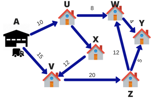
Suppose you've got six packages delivered daily by a FedEx courier. The warehouse is at point A. The six destinations are indicated by U, V, W, X, Y, Z. The numbers on the road indicate the space between cities. To save lots of fuel and time, delivery personnel want to use the shortest route.

           Fig 1

Therefore, the courier calculates different routes to succeed in all six destinations and comes up with the shortest route. This method of selecting the littlest way is named applied mathematics.

In this case, the deliveryman's purpose is to deliver the parcel to all or any six destinations on time. The method of selecting the simplest route is named research. Research may be a decision-making approach that has a group of methods for operating a system. Within the example above, my system was a delivery model.

Linear programming is employed to seek out the optimal solution to a given constrained problem. Applied mathematics formulates a true problem into a mathematical model. This includes objective functions and linear inequalities that are subject to constraints.

Does the 6-point linear representation above represent the important world? Yes, No. the particular route isn't a line, so it's oversimplified. Multiple turns, U-turns, traffic lights, and traffic jams can occur. However, with simple assumptions, we are creating an answer that greatly reduces the complexity of the matter and works in most scenarios.

• Applications of LP

Linear programming and optimization are used in a variety of industries. Manufacturing and service industries regularly use linear programming.

1. Manufacturing uses linear programming to analyse supply chain operations.  Their motivation is to maximize efficiency with minimal operating costs. Following the recommendations of the linear programming model, manufacturers can reconfigure their storage layouts and adjust their employees to reduce bottlenecks. This is a case study of Cequent's small warehouse based in the United States. Watch this video for a clearer understanding.
2. Linear programming is also used in retail stores organized to optimize shelf space. With the number of products on the market growing exponentially, it's important to understand what your customers want. Optimization is actively used in stores such as Wal-Mart, Hyper city, Reliance, and Big Bazaar. The products in the store are strategically placed with the customer's shopping patterns in mind. The goal is to make it easier for customers to find and select the right product. This has limitations such as limited shelf space and various products.
3. Optimization is also used to optimize delivery routes. The service industry uses optimization to find the best route for multiple salespeople travelling to multiple cities. With the help of clustering and greedy algorithms, delivery routes are determined by companies such as FedEx and Amazon. The goal is to minimize operational costs and time.
4. Optimization is also used in machine learning. Supervised learning addresses the basics of linear programming. The system is trained to fit a mathematical model of a function from labelled input data that can predict values   from unknown test data.

The application of linear programming does not end here. There are many other real-world linear programming applications, such as those applied by shareholders, sports, stock markets, and more. Please continue to explore further.

• Components of LP

General terminology utilized in applied mathematics

Let's use the instance above to define some terms utilized in applied mathematics.

Determinants: Determinants are variables that determine the output. They represent my ultimate solution. To unravel the matter, you initially got to identify the coefficient of determination. Within the above example, the entire number of units A and B, represented by X and Y, respectively, is my coefficient of determination.

Objective function: Defined because the objective of deciding. Within the example above, the corporate wants to extend the gross profit margin, represented by Z. Therefore, profit is my objective function.

Constraint: A constraint may be a limit or limit on a choice variable. These usually limit the worth of the choice variable. Within the above example, limiting the supply of Milk and Chocó resources is my constraint.

Non-negative limit: altogether applied mathematics, the choice variable should take a non-negative value. This suggests that the worth of the choice variable must be greater than or adequate to 0.

The process of formulating an applied mathematics problem

Let's take a glance at the steps to generally define an applied mathematics problem.

1. Identify the coefficient of determination
2. Write an objective function
3. Mention constraints
4. Explicitly state non-negative limits

For the matter to be an applied mathematics problem, the choice variables, objective functions, and constraints must all be linear functions.

If all three conditions are met, it's called an applied mathematics problem.

In order for the corporate to form the foremost profit, the above inequality must be met. When converted into a mathematical model is called formulating a real-world problem

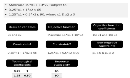
The other two factors are resource availability and technical factors. These can be better explained using the example below. The executable solution of a linear programming problem must meet the constraints and non-negative constraints. The executable solution of LPP with the maximization problem is the optimal solution when the objective function value is maximum (maximum). Similarly, an LPP executable solution with a minimization problem is optimal when the objective function value is the minimum (minimum).

                                               Fig 2 Elements of LPP

• Requirements for Formulation of LP Problem

Problem Formulation-Let's Make Some Chocolate

Example: Consider a chocolate manufacturer that produces only two sorts of chocolate, A and B. Both chocolates only require milk and chocolate. To manufacture each of the A and B units, you would like the subsequent quantities:

Each unit during a requires 1 unit of milk and three units of chocolate

Each unit in B requires 1 unit of milk and a couple of units of chocolate.

The company's kitchen features a total of 5 units of milk and 12 units of chocolate. With each sale, the corporate makes a profit

Rs6 per unit A sold

Rs5 per unit B sold.

Now the corporate wants to maximise profits. What percentage units of A and B does one got to produce respectively?

Solution: the primary thing to try to is to tabulate the matter for better understanding.

Let = X be the entire number of units generated by A.

Let = Y be the entire number of units generated by B.

Now, the entire profit is represented by Z

The company's gross profit margin is that the total number of A and B units produced multiplied by the profit per Rs6 and Rs5 units, respectively.

Profit: Maximum Z = 6X + 5Y

That is, you would like to maximize Z.

The company will attempt to produce as many A and B units as possible to maximize profits. However, Milk and Chocó resources are available in limited quantities.

As shown within the table above, each unit A and B requires 1 unit of milk. The entire amount of milk available is 5 units. To precise this mathematically,

X + Y ≤ 5

Also, each unit A and B requires 3 units and a couple of units of Chocó, respectively. The entire number of chocolates sold is 12. To precise this mathematically,

3X + 2Y ≤ 12

Also, the unit value of A can only be an integer.

Therefore, there are two constraints, X ≥ 0 and Y ≥ 0.

• Assumptions Underlying Linear Programming

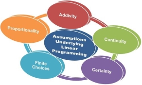
There are some assumptions that linear programming works, these are:

Fig 3

1. Proportional: The basic assumption underlying linear programming is that as the constraint inequality changes, so does the objective function. That is, if the product provides Rs 20 for profit, the total contribution is equal to 20x1. Where x1 is the number of units in the product.

For example, if the product has 5 units, the contribution will be Rs 100, and if it has 10 units, it will be Rs 200. Therefore, if the output (sales) is doubled, the profit is also doubled. ..

2.     Additivity: The additive assumption argues that the total profit of the objective function is determined by the sum of the profits provided individually by each product. Similarly, the total amount of resources used is determined by the total amount of resources each product uses individually. This means that there is no interaction between the decision variables.

3.     Continuity: Another assumption of linear programming is that the coefficient of determination is continuous. This means that you can use a combination of outputs with integer values   as well as decimal values.

For example, if 52/3 units of product A and 10 1/3 units of product B are produced in a week. In this case, a fraction of production is considered work in progress and the remaining production portion is acquired the following week. Therefore, producing 17 units of product A and 31 units of product B in 3 weeks means 52/3 units of product A and 10 1/3 units of product B per week

4.     Certainty: Another basic assumption of linear programming is certainty. That is, the coefficients of the objective function coefficient parameters and the constraint inequality are definitely known. The profit per unit of a product, the availability of materials and workforce per unit, the requirements for materials and workforce per unit, etc. are known and given in a linear programming problem.

5.     Finite choice: This assumption means that the decision maker has a particular choice and the decision variable assumes a non-negative value. The non-negative assumption is true in a sense, and the output of a production problem cannot be negative. Therefore, this assumption is considered feasible.

Therefore, when solving a linear programming problem, you need to keep these assumptions in mind so that the best alternative is selected.

• Steps in Solving LP Problems

The steps involved in forming a linear programming problem are as follows:

Step 1 → Identify the decision variables that the decision maker is interested in and represent them as x1, x2, x3 ………

Step 2 → Determine the purpose for the decision maker to decide whether to minimize or maximize.

Step 3 → Check the cost (for minimization problem) or profit (for maximization problem) per unit of each decision variable.

Step 4 → Check the constraints that represent maximum availability or minimum commitment or equivalence and represent them as less than or equal to (≤) type inequalities or greater than or equal to (≥) type inequalities or as "equal" (=) type equivalence.

• LPP Formulation (Decision Variables, Objective Function, Constraints, Non Negativity Constraints)

Formulation of applied mathematics model

The three components are:

1. Coefficient of determination

2. Environmental (out of control) parameters

3. Result (dependent) variable

The applied mathematics model consists of equivalent components

Terminology utilized in applied mathematics problems

1. LP Problem Components: All LPPs are made from the coefficient of determination,

b. Objective function,

c. Constraints.

2. Optimization: applied mathematics attempts to maximise or minimize the worth of the target function.

3. Cost Factor Benefit: The coefficient of the target function variable represents the speed at which the worth of the target function increases or decreases by including one unit of every decision variable within the solution.

Coefficient of determination

Objective function

Constraint

4. Constraints: Maximization (or minimization) is performed consistent with a group of constraints. Therefore, LP is often defined as a constrained optimization problem. They reflect

Resource limits.

5. Input / output coefficient: The coefficient of the constraint variable is named the input / output coefficient. These indicate the speed at which a specific resource is unitized or depleted. They are showed the left of the constraint.

6. Capacity: The capacity or availability of varied resources is shown to the proper of the constraint.

Key takeaways:

1. Optimization may be a way of life. We all have limited resources and time and need to form the foremost of them.
2. Applied mathematics may be a simple technique that uses linear functions to represent complex relationships and find the simplest points. The important words within the preamble are drawn.
3. Linear programming applications are everywhere around you. Use applied mathematics on a private and professional side.
4. Linear programming is employed to seek out the optimal solution to a given constrained problem.
5. Linear programming and optimization are used in a variety of industries.
6. The application of linear programming does not end here. There are many other real-world linear programming applications, such as those applied by shareholders, sports, stock markets, and more.
7. Let's use the instance above to define some terms utilized in applied mathematics.
8. For the matter to be an applied mathematics problem, the choice variables, objective functions, and constraints must all be linear functions.
9. Therefore, when solving a linear programming problem, you need to keep these assumptions in mind so that the best alternative is selected.

1.3    Linear Programming Problems: Graphical Method

• Maximization & Minimization Type Problems. (Max. Z & Min. Z)
• Two Decision Variables and Maximum Three Constraints Problem
• Constraints can be “less than or equal to”, “greater than or equal to” or a combination of both the types i.e. mixed constraints.

Concepts: Feasible Region of Solution, Unbounded Solution, Redundant Constraint, Infeasible Solution, Alternative Optima

Solve applied mathematics during a graphical way

Linear programming is often solved in multiple ways. During this section, we'll check out graphical thanks to solve applied mathematics. This method is employed to unravel two-variable applied mathematics. If you've got only two decision variables, you would like to use a graphical method to seek out the simplest solution.

The graphical method formulates a group of linear inequalities that are subject to constraints. The inequality is then plotted on the XY plane. If you plot all the inequalities on a graph, the intersecting regions offer you a feasible region. The Feasible region describes all the values a model can take. And it also gives us the simplest solution.

Let's understand this with an example.

Example: A farmer recently acquired 110 hectares of land. He decided to grow wheat and barley there. The standard of the sun and therefore the excellent climate of the region allow us to sell all wheat and barley products. He wants to understand the way to plant each variety on 110 hectares, taking under consideration costs, net, and labor requirements, consistent with the info shown below.

The farmer's budget is US $ 10,000 and 1,200 man-days are available during the design period. Find the optimal solution and value.

Solution: to unravel this problem, first create a applied mathematics method.

Formulation of linear problems

Step 1: Identify the coefficient of determination

Total area for growing wheat = X (hectare)

Total area for growing barley = Y (hectare)

X and Y are my coefficients of determination.

Step 2: Write the target function

As we can sell products from the whole land to the market. The farmer will want to maximize the profits of his total product. You’ll tend internet profit of both wheat and barley. Farmers earn a net income of $ 50 per hectare of wheat and $ 120 per hectare of barley.

Our objective function (given by Z) is up to Z = 50X + 120Y.

Step 3: Write constraints 

1. The entire budget of farmers is estimated to be US $ 10,000. The value of manufacturing wheat and barley per hectare is additionally given to us. There’s an upper limit to the entire cost a farmer can spend. Therefore, the equation is:

100X + 200Y ≤ 10,000

2. The subsequent constraint is that the upper limit of availability of total man-hours during the design period. The entire number of construction days available is 1200. As shown within the table, the man-hours per hectare of wheat and barley are shown.

10X + 30Y ≤ 1200

3. The third constraint is that the total acreage present within the plantation. The entire area available is 110 hectares. Therefore, the equation is:

X + Y ≤ 110

Step 4: Non-negative limit

The X and Y values are greater than or adequate to 0. to not mention this.

X ≥ 0, Y ≥ 0

We have formulated a applied mathematics method. it is time to unravel it.

Solve LP during a graphical way

We know that X, Y ≥ 0, so consider only the primary quadrant.

To plot the graph of the above equations, first simplify all the equations.

100X + 200Y ≤ 10,000 are often simplified to X + 2Y ≤ 100 by dividing by 100.

10X + 30Y ≤ 1200 are often simplified to X + 3Y ≤ 120 by dividing by 10.

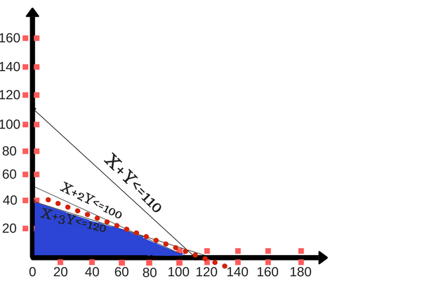
The third equation may be a simplified sort of X + Y ≤ 110. Plot the primary two lines on the graph in quadrant 1 (see below)

Optimal feasible solutions are achieved at intersections where budget and man-hour constraints are active. This suggests that the purpose where the equations X + 2Y ≤ 100 and X + 3Y ≤ 120 intersect gives the optimal solution.

The values of X and Y that give the optimal solution are (60,20).

To increase profits, farmers got to manufacture wheat and barley on 60 hectares and 20 hectares of land, respectively.

The biggest profit the corporate gets is

Maximum Z = 50 * (60) + 120 * (20)

= US $ 5400

Solve the following LPP graphically-

Maximize-

Subject to the constraints-

Sol.

Change the given constraints into equations-

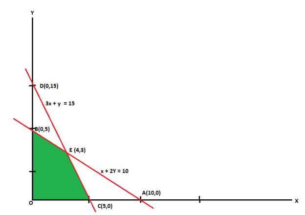
The line   meets the x-axis at the point A(10,0) and meets the y-axis at the point B(0,5). Join A and B to get the graph for the line.             

Hence origin (0,0) satisfies the inequality so that half plane containing the origin represent the solution set of .

And

The line meets the x-axis at the point C(5,0) and meets the y-axis at the point D(0,15). Join C and D to get the graph for the line.

Hence origin (0,0) satisfies the inequality   so that half plane containing the origin represent the solution set of.

Now all the points in first quadrant satisfies  .

So that first quadrant is the region represented by

Hence the region OCEBO satisfies all the inequalities.

And each point on the region is the feasible solution of the problem.

Feasible solution-

Here in this problem the feasible solution is (5,0), (4,3) and (0,5).

Now we can obtain the optimal solution of the problem.

As we know that any point in the feasible region that gives the optimal value is called an optimal solution.

The value of the objective function at corner points of the feasible region is given below-

Here we see that the maximum value of Z is 18.

Find the maximum value of Z = 2x + 3y subject to the constraints-

Sol.

Any point (x,y) satisfying the conditions lies in the first quadrant only.

Also since the desired point (x,y) lies within the convex region ABCDE.

Its vertices are A(3,3), B(20,3), C(20,10), D(18,12) and E(12,12).

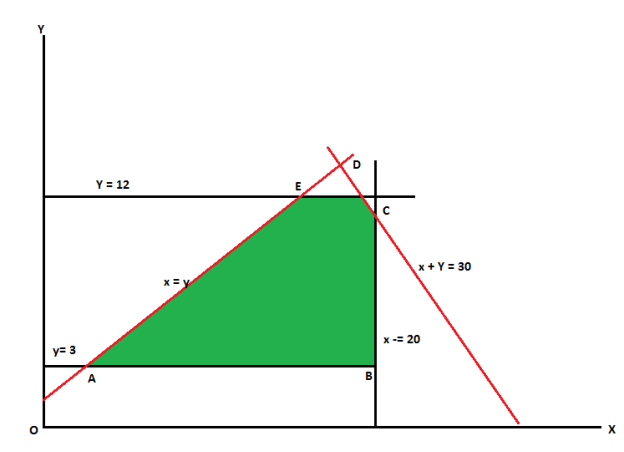
The value of Z at these points are-

Z(A) = 15

Z(B) = 49

Z(C) = 70

Z(D) = 72

Z(E) = 60

Here 72 is the maximum value which is at D.

So that the solution of the LPP is x = 18 and y = 12 and maximum Z  = 72

Example: A factory manufactures two types of items, A and B, each type requiring the use of two machines, an automatic and a hand operated. It takes 4 minutes on the automatic and 6 minutes on hand operated machines to manufacture a package of item A, while it takes 6 minutes on automatic and 3 minutes on the hand operated machines to manufacture a package of item B. Each machine is available for at the most 4 hours on any day. The manufacturer can sell a package of item A at a profit of Rs. 7 and item B at a profit of Rs 10. Assuming that he can sell all the items he manufactures, how many packages of each type should the factory owner produce in a day in order to maximize his profit ?

Determine the maximum profit.

Solution

We can tabulate the data as follows-

Decision variables- Let the manufacturer produce x packages of item A and y packages of item B per day respectively.

Objective function- Suppose Z denotes the maximum profit,

Constraints-

1st constraint-

2nd constraint-

3rd constraint-

Mathematical formulation-

The mathematical form of this LPP can be written as-

Maximize
 

Subject to the constraints-

Tables for the region represented by inequalities-

For the first constraint-

For second condition-
 

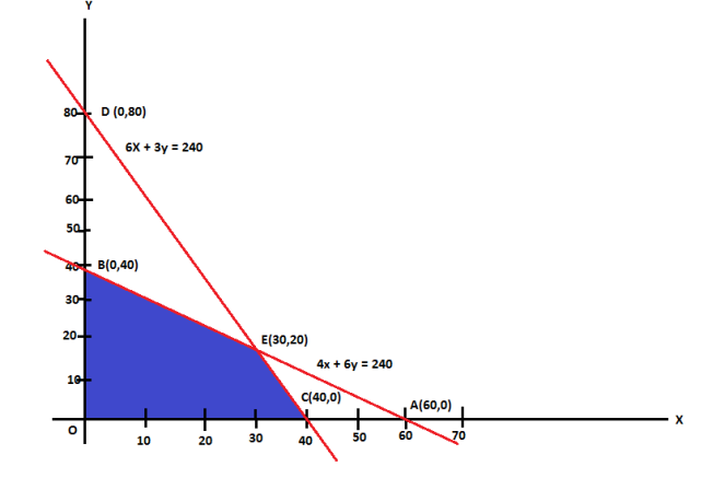
Now we draw on x and y axes.

The coordinates of the vertices O, C, E and B of the feasible region OCEBO are O (0, 0), C (40, 0), E (30, 20) and B (0, 40). The coordinates of E are obtained by solving the equations 4x + 6y = 240 and 6x + 3y = 240.             

Therefore Z is maximum at x = 30 and y = 20 and the maximum value of Z is 410.

Note: Everything taught here is additionally taught within the course format of this free course-an applied mathematics method for data science professionals.

Key takeaways:

1. Linear programming is often solved in multiple ways. During this section, we'll check out graphical thanks to solve applied mathematics.
2. The graphical method formulates a group of linear inequalities that are subject to constraints. The inequality is then plotted on the XY plane.
3.  If you plot all the inequalities on a graph, the intersecting regions offer you a feasible region.

   1.4 Linear Programming Problems: Simplex Method

   Simplex method

The simplex method is one of the most powerful and popular linear programming methods. The simplex method is an iterative procedure to get the most viable solution. This method keeps transforming the values   of the fundamental variables to get the maximum value of the objective function.

Linear programming functions are in standard form when trying to maximize the objective function. Subject to constraints,

Here and after adding the Slack variable, the system of corresponding constraint equations

Where,

……………….is called a slack variable. These are non-negative numbers that are added to remove the inequality from the equation.

The above explanation is a theoretical explanation of the simplex method. Next, I will explain how to actually use the simplex method using Excel.

Example: Company alternative ads include TV, newspaper, and radio ads. The cost of each media, including audience coverage, is as follows:

Local newspapers limit the number of ads from one company to 10. In addition, less than half of the total number of ads must occur on the radio in order to balance the ads among the three media types. And at least 10% should happen on TV. The weekly advertising budget is $ 18,200. How many ads do you need to run on each of the three media types to maximize your total audience?

Solution: First, formulate the problem for a clear understanding.

Step 1: Identify decision variables

, , Represent the total number of TV, newspaper and radio ads, respectively.

  Step 2: Objective function

The purpose of the company is to maximize the audience. The objective function is given by the following equation.

   Step 3: Make a note of the constraints

   Now let's look at each constraint one by one.

Clearly there are budget constraints. The total budget that can be allocated is $ 18,200. Also, the individual costs per TV, newspaper, and radio ad are $ 2000, $ 600, and $ 300, respectively. This can be expressed by the following formula.

   For newspaper ads, the maximum number of ads is 10. My first constraint is     

The next constraint is the number of TV ads. The company wants at least 10% of all ads to appear on TV. Therefore, it can be expressed as: 

The final constraint is that the number of ads on the radio cannot exceed half the total number of ads. It can be expressed as

You have now formulated a linear programming problem. The simplex method is used to solve this. I will introduce the simplex method one by one.

Again, all the constraints are: We have simplified the last two equations into a standard format.

There are a total of four equations. Introduce four slack variables,,and to balance each equation.

I hope you can understand the whole problem of advertising. All of the above formulas are for a better understanding. Solving these equations yields the values   X1 = 4, X2 = 10, and X3 = 14.

Solving the objective function yields a maximum audience of 1,052,000 per week. You can solve the equation by following this tutorial. Follow this tutorial to solve linear programming in Excel.

Example: Maximize

Subject to-

By using simplex method.

Sol. Here all b’s are positive and the objective function is to be maximized.

Step-1: Now express the problem in the standard form-

Let are slack variables then the problem in standard form becomes-

Maximize-

Subject to

Step-2: find the initial basic feasible solution-

There are three equations having 5 unknowns and for obtaining the solution we assign zero value to any two of the three variables.

We start with a basic solution for which we set and .

Putting  

in the above three equations-

We get-

Here all
are positive, the basic solution is also feasible and non-degeneate.

The BFS is-

Initial BFS is given by the table below-

For

For

Similarly-

Now apply the optimality test-

As is positive under some columns, the IBFS is not optimal, we move to the next step-

Step- Identify the outgoing and incoming variables-

By the above table is the incoming variable as its incremental contribution is max. And the column in which it appears is the key column.

Dividing the  elements under b-column by the corresponding elements of key-column we find the mi. Positive ratio in two rows.

Therefore we arbitrarily choose the row containing as the key row.

The elements at the intersection of key row and the key column is the key element.

is therefore the outgoing variable which will now become non-basic.

Having decided that is to enter the solution we have tried to find as to what maximum under could have without violating the constraints.

So that removing , the new basis will contain as the basic variables.

Now iterate towards the optimal solution-

To transform the initial set of equations with a BFS into an equivalent set of equations with a different BFS, we make the key element unity.

We retain the key row as it is. Then to make all other elements in key column zero, we subtract proper multiples of the key row from the other rows.

Here we subtract five times the elements of key row from the second row and three times the element of key row from the third row.

These become the second and the third of the next table.

We also change the corresponding value under column from 0 to 5.

While relacing by under the basis.

Thus the second BFS is given below-

As is either zero or negative under all columns, the above table gives the optimal BFS.

This optimal BFS is-

Example: Maximize-

Subject to-

By using simplex method.

Sol.

Here we have

And  the inequalities-

...... (1)

........ (2)

  ..........(3)

By adding we get-

  ...... (4)

....... (5)

...... (6)

Putting decision variables equals to zero, we get-

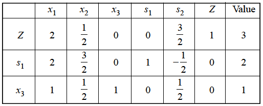
Since coefficient (–3) of is most negative, so x3 is entering variable.

The smallest ratio is 1 in the s2-row, therefore s2 is departing variable. The pivot entry (2) is at the intersection of x3-column and s2-row.

To make pivot entry (1), we multiply third row by ½, we get-

Applying R1 R1 + 3R3 and R2 R2 - R1, we get

Since, Z row of the table has non-negative entries in the column of variables, therefore, this is the case of optimal solution. From the last column of the table we have x1 = 0, x2 = 0 and x3 = 1 and the maximum value of Z = 3.

Key takeaways:

1. The simplex method is one of the most powerful and popular linear programming methods.
2. The simplex method is an iterative procedure to get the most viable solution. This method keeps transforming the values   of the fundamental variables to get the maximum value of the objective function.
3. Linear programming functions are in standard form when trying to maximize the objective function.

References:

1. Higher engineering mathematics, B.S. gerewal
2. Hk dass