4.1 Monopoly: Monopoly short run and long run equilibrium

The word monopoly has been derived from the combination of two words i.e., ‘Mono’ and ‘Poly’. Mono refers to a single and poly to control.

Thus, monopoly refers to a market situation in which there is only one seller of a commodity.

In monopoly market, single firm or one seller controls the entire market. The firm has all the market power, so he can set the prices to earn more profit as the consumers do not have any alternative.

Definition

“Pure monopoly is represented by a market situation in which there is a single seller of a product for which there are no substitutes; this single seller is unaffected by and does not affect the prices and outputs of other products sold in the economy.” Bilas

“Monopoly is a market situation in which there is a single seller. There are no close substitutes of the commodity it produces, there are barriers to entry”. –Koutsoyiannis

“A pure monopoly exists when there is only one producer in the market. There are no dire competitions.” –Ferguson

Features

2.     No Close Substitutes - There is no close substitutes for the product sold by the monopolist. The cross elasticity of demand between the product of the monopolist and others must be negligible or zero.

3.     Difficulty of Entry of New Firms - There are restrictions on the entry of firms into the industry, even when the firm is making abnormal profits. Other sellers are unable to enter the market of the monopoly

4.     Profit maximizer: a monopoly maximizes profits. Due to the lack of competition a firm can charge a set price above what would be charged in a competitive market, thereby maximizing its revenue.

5.     Price Maker - Under monopoly, monopolist has full control over the supply of the commodity. The price is set by determining the quantity in order to demand the price desired by the firm. Therefore, buyers have to pay the price fixed by the monopolist.

Monopoly short run and long run equilibrium

Short run

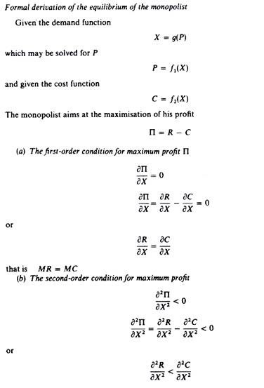
A monopolist maximizes his short-term profits if the following two conditions are met first, MC equals Mr. Secondly; the slope of MC is larger than that of Mr at the intersection.

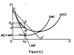
In Figure 6.2, the equilibrium of the monopoly is defined by the point θ at which MC intersects the MR curve from below. Thus, both conditions of equilibrium are met. The price is PM and the quantity is XM. Monopolies realize excess profits equal to shaded areas APM CB. Please note that the price is higher than Mr

In pure competition, the company is the one who receives the price, so it’s only decision is the output decision. The monopolist is faced with two decisions: to set his price and his output. But given the downward trend demand curve, the two decisions are interdependent.

Monopolies set their own prices and sell the amount the market takes on it, or produce an output defined by the intersection of MC and MR and are sold at the corresponding price. An important condition for maximizing the profits of monopolies is the equality of the MC and the MR, provided that the MC cuts the MR from below.

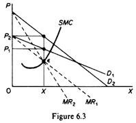
We can now revisit the statement that there is no unique supply curve for the monopolist derived from his MC. Given his MC, the same amount could be offered at different prices depending on the price elasticity of demand. This is graphically shown in Figure 6.3. Quantity X is sold at price P1 if demand is D1, and the same quantity X is sold at price P2 if demand is D2.  

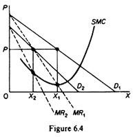
So there is no inherent relationship between price and quantity. Similarly, given the monopolist MC, we can supply various quantities at any one price, depending on the market demand and the corresponding MR curve. Figure 6.4 illustrates this situation. The cost condition is represented by the MC curve. Given the cost of a monopolist, he would supply 0X1 if the market demand is D1, then p at the same price, and only 0X2 if the market demand is D2 B.Long-term equilibrium:

Long run

In the long run the monopolist will have time to expand his plants or use his existing plants at every level to maximize his profits. However, if the entry is blocked, the monopolist does not need to reach the optimal scale (that is, the need to build the plant until the minimum point of LAC is reached), neither does the guarantee that he will use his existing plant at the optimum capacity. What is certain is that if he makes a loss in the long run, the monopolist will not stay in business.

He will probably continue to earn paranormal benefits even in the long run, given that entry is banned. But the size of his plant and the degree of utilization of any plant size depends entirely on the market demand. He may reach the optimal scale (the minimum point of Lac), stay on the less optimal scale (the falling part of his LAC), or exceed the optimal scale (expand beyond the minimum LAC), depending on market conditions.

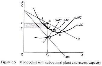
Figure 6.5 shows when the market size does not allow the monopolist to expand to the minimum point of Lac. In this case, not only is his plant not optimal (in the sense that the economy of full size is not depleted), but also the existing plant is not fully utilized. This is because on the left of the minimum point of the LAC, the SRAC touches the LAC at its falling part, and the short-term MC must be equal to the LRMC. This happens in e, but the minimum LAC is b,and the optimal use of the existing plant is a. Since it is utilized at Level E', there is excess capacity.                                                                Finally, figure 6.7 shows a case where the market size is large enough for a monopolist to build an optimal plant and be able to use it at full capacity.

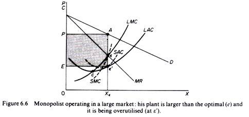
In Figure 6.6, the scale of the market is so large that monopolists have to build plants larger than the optimal ones to maximize output and over-exploit them. This is because to the right of the minimum point of LAC, SRAC and LAC is tangent at the point of positive slope, and SRMC must be equal to LAC. Thus, plants that maximize the profits of monopolies are, firstly, larger than the optimal size, and secondly, they are over-utilized, which leads to higher costs. This is often the case with utility companies operating at the state level.     

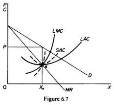
It should be clear that which of the above situations will appear in a particular case will depend on the size of the market (given the technology of monopolists). There is no certainty that monopolies will reach their optimal size in the long run, as is the case with purely competitive markets. In Monopoly, there is no market force similar to those of pure competition that will lead companies to operate at optimal plant size in the long run (and utilize it at its full capacity).

Price determination

A monopolistic firm is a price-maker, not a price-taker. Therefore, a monopolist can increase or decrease the price. Also, when the price changes, the average revenue, and marginal revenue changes too. Take a look at the table below:

Let’s look at the revenue curves now:

As you can see in the figure above, both the revenue curves (Average Revenue and Marginal Revenue) are sloping downwards. This is because of the decrease in price. If a monopolist wants to increase his sales, then he must reduce the price of his product to induce:

• The existing buyers to purchase more

• New buyers to enter the market

Hence, the demand conditions for his product are different than those in a competitive market. In fact, the monopolist faces demand conditions similar to the industry as a whole.

Therefore, he faces a negatively sloped demand curve for his product. In the long-run, the demand curve can shift in its slope as well as location. Unfortunately, there is no theoretical basis for determining the direction and extent of this shift.

Talking about the cost of production, a monopolist faces similar conditions that a single firm faces in a competitive market. He is not the sole buyer of the inputs but only one of the many in the market. Therefore, he has no control over the prices of the inputs that he uses.

Role of time element in determination of price are given below:

Time plays an important role in the theory of volume, i.e., price determination because supply and demand conditions are affected by time.

Price during the short-period can be higher or lower than the cost of production, but in the long-period price will have a tendency to be equal to the cost of production.

The relative importance of supply on demand in the determination of price depends upon the time given to supply to adjust itself to demand.

To study the relative importance of supply or demand in price determination, Prof. Marshall has divided time element-into three categories:

(a) Very short period or market period.

(b) Short period.

(c) Long period.

(a) Very short period (determination of market price):

Market period is a time period which is too short to increase production of the commodity in response to an increase in demand. In this period the supply cannot be more than existing stock of the commodity.

The supply of perishable goods is perfectly inelastic during market period. But non-perishable goods (durable goods) can be stored.:

Therefore, the supply curve of non-perishable goods above reserve price has a positive scope at first but becomes perfectly inelastic after some price level.

The reserve price y depends upon-(i) cost of storing, (ii) future expected price, (iii) future cost of production, and (iv) seller’s need for cash we will discuss the determination of market price by taking a perishable commodity and determination of market price is illustrated.

DD is the original demand curve and SS the market period supply curve. The demand curve DD (perfectly inelastic) cuts the supply curve SS at point E. Point E, is the equilibrium point and equilibrium price is determined at OP, level.

Increase in demand shifts the demand curve to D,D and the price also increased to OP,. Decrease in demand shifts the demand curve downward to D2D2 and the price too falls to OP It is, thus, clear that in market period price fluctuates with change in demand conditions.

(b) Price determination is short period:

In the short period fixed factors of production remain unchanged, i.e., productive capacity remains unchanged.

However, in the short period supply can be affected by changing the quantity of variable factors.

In other words, during the short period supply can be increased to some extent only by an intensive use of the existing productive capacity.

Therefore, the supply curve in the short-run slopes positively, but the supply curve is less elastic. Determination of price in the short-run is illustrated.

SS is the market period supply curve and SRS is short-run supply curve. The original demand curve DD cuts both the supply curves at E, point and thus OP, price is determined.

Increase in demand shifts the demand curve upward to the right to D,D,. Now with the increase in demand the market price (in market period) rises at once to OP3 because supply remains fixed. But in the short-run supply increases. Therefore, in the short-run price will cuts the SRS curve. If demand decreases opposite will happen.

(c) Price determination in long period (Normal Price):

In the long period there is enough time for the supply to adjust fully to the changes in demand.

In the long period all factors are variable. Present firms can increase on decrease the size of their plants (productive capacity).

The new firms can enter the industry and old firms can leave the market. Therefore, long-period supply curve has a positive slope and is more elastic than short period supply curve.

The shape of supply curve of the industry depends upon the nature of the laws of returns applicable to the industry. Price determination in the long period is illustrated.

DD is the original demand curve and LS is the long period supply curve of the industry. Demand curve DD and supply curve LS both intersect each other at E point and OP price is determined.

This price will be equal to minimum average cost (AC) of production because in the long period firms under perfect competition can only earn normal profits. Suppose these are permanent increase in demand.

With the increase in demand, the demand curve shifts to D1,D1. As a result of increase in demand the price in the market period and short period will rise.

Due to increase in price present firms will earn above normal profit. Therefore, new firms will enter into market in the long period.

As a result of it supply will increase in the long period. In the long period price will be determined at OP1, level because at this price demand curve D1 D2 cuts the LS curve at E2 point.

Price OP1, is greater than previous price OP1, because the industry is an increasing cost industry. This new higher price will also be equal to minimum average cost of production

Key takeaways –

4.2 Shifts in demand curve and the absence of the supply curve

Shifts in demand curve:

A demand curve is a line or a curve showing the relationship between the quantity purchased and their respective prices. A normal demand curve will slope from the left to the right. This is said to be the demand curve for normal goods. There are exceptional like the demand curve for inferior goods or giffen goods that does not follow this principle. The demand curve for inferior goods for example will have a zero gradient since the changes in prices will not affect the quantity demanded from the market. The demand curve whether it is normal or abnormal has certain unique features. For example the demand curve can make some movements on the Cartesian planes when the various factors that influence the quantity demanded are varied. The movement can either be along the demand curve or movement away fro the original demand curve. Movement along the demand curve is referred to by economists as either expansion or contraction. The upwards movement along the demand curve is called contraction and the downwards movement along the demand curve is called expansion. Movement along the demand curve is caused only by changes in commodities prices.

Our main interest on the movement of demand curves is the shift in the demand curve. The shift in demand curve is caused by the other factors that influence demand apart from the price changes. For the shift in demand curve to occur all the other factors must be changing but the prices has to remain the same. The shift in the demand is referred to as a change in consumers demand. The major factors that result to the shift in demand curve are; changes in the consumer’s income, changes in consumer’s expectation or speculation, changes in the prices or related goods related goods can be grouped as either complimentary goods or substitute’s goods. Complimentary goods are goods that are consumed together. One good cannot be used on its own. An example is car and fuel. Substitute goods are goods that are used to satisfy the same need or want. The last major factor that results to a shift in demand curve is the changes in consumer’s tastes and preference.

An increase in consumer’s income will cause two types of changes depending of the type of goods being purchased by the consumers. When an increase in the consumers income results in an upwards shift on the demand curve that type of good is referred to as a normal goods. It means that increase in consumer’s purchasing power increases the demand for that commodity. The second type of good is an inferior good. An increase in consumer’s wealth will reduce the quantity demanded from that commodity. It means that consumers will only purchase that product under budget constraints. Taste and preference is another factor that results to a shift in demand curve. Loss in consumers taste and preference for ac certain commodity will result to a downward movement of demand curve. Fashion is an example that result to either loss or increase in preference for a commodity. The demand curve for a good that is in fashion will shift upwards provide prices are kept constant

Absence of the supply curve:

The supply curve of a product by a firm traces out the unique price-output relationship, that is, against a given price there is a particular amount of output which the firm will produce and sell in the market. The concept of supply curve is relevant only when the firm exercises no control over the price of the product. As price changes due to the shift in demand, the competitive firm equates the new higher price (i.e. new MR) with its marginal cost at higher level of output. In this way under perfect competition, marginal cost curve becomes the supply curve of the firm.

Key takeaways –

4.3 Measurement of monopoly power and the rule of thumb for pricing, Horizontal and vertical integration of firms

Measurement of monopoly power and the rule of thumb for pricing:

Monopoly Power

- Monopoly is rare.

- However, a market with several firms, each facing a downward sloping demand curve will produce so that price exceeds marginal cost.

• Measuring Monopoly Power

- Perfect competition: P = MR = MC

- Monopoly power: P > MC

- Lerner’s Index of Monopoly Power : L = (P - MC)/P

- The larger the value of L ( 0 < L< 1), the greater the monopoly power.

- L is expressed in terms of Ed : L = (P - MC)/P = -1/Ed

- Ed is elasticity of demand for a firm, not the market.

Thumb Rule:

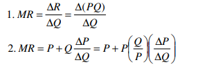
A Rule of Thumb for Pricing in Monopoly

Horizontal and vertical integration of firms:

Vertical integration is the process in which several steps in the production and/or distribution of a product or service are controlled by a single company or entity, in order to increase that company’s or entity’s power in the marketplace.

Simply said, every single product that you can think of has a big life cycle. While you might recognize the product with the Brand name printed on it, many companies are involved in developing that product. These companies are necessarily not part of the brand you see.

Example of vertical integration: while you are relaxing on the beach sipping chilled cold drink, the brand that you see on the bottle is the producer of the drink but not necessarily the maker of the bottles that carry these drinks. This task of creating bottles is outsourced to someone who can do it better and at a cheaper cost. But once the company achieves significant scale it might plan to produce the bottles itself as it might have its own advantages (discussed below). This is what we call vertical integration. The company tries to get more things under their reign to gain more control over the profits the product / service delivers.

Types of Vertical Integrations:

There are basically 3 classifications of Vertical Integration namely:

1. Backward integration – The example discussed above where in the company tries to own an input product company. Like a car company owning a company which makes tires.

2. Forward integration – Where the business tries to control the post production areas, namely the distribution network. Like a mobile company opening its own Mobile retail chain.

3. Balanced integration – You guessed it right, a mix of the above two. A balanced strategy to take advantages of both the worlds.

Horizontal Integration

Much more common and simpler than vertical integration, Horizontal integration (also known as lateral integration) simply means a strategy to increase your market share by taking over a similar company. This takes over / merger / buyout can be done in the same geography or probably in other countries to increase your reach.

Examples of Horizontal Integration are many and available in plenty. Especially in case of the technology industry, where mergers and acquisitions happen in order to increase the reach of an entity.

Key takeaways –

Sources