UNIT 3
Inflation and Unemployment
Inflation is a rate of change in the price level. The rate of change is measured with reference to the base year so that a long term perspective is obtained with regard to price rise. For all practical purposes, inflation rate is measured on yearly basis. However, in recent years, the inflation rate is also measured on monthly and weekly basis. The rate of inflation can be measured as: P = (P - P0)/P0 *100
Demand pull inflation
Definition
Demand-pull inflation exists when aggregate demand for a good or service exceeds aggregate supply. It starts with an increase in consumer demand. Sellers meet such an increase with more supply. But when additional supply is unavailable, sellers raise their prices. That results in demand-pull inflation.
When there is excess demand in the economy, producers are able to raise prices and achieve bigger profit margins because they know that demand is running ahead of supply. Typically, demand-pull inflation becomes a threat when an economy has experienced a strong boom with GDP rising faster than the long run trend growth of potential GDP.
Demand pull inflation takes place due to rise in aggregate demand. Aggregate demand may rise due to combined effect of higher demand from the various sectors of the economy such as the firms, households and the government. According to Keynes, inflation arises when there is an inflationary gap in the economy. Inflationary gap arises when aggregate demand is greater than aggregate supply at full employment level of output. Keynes explained inflation in terms of demand pull forces. When the economy is operating at the full employment level of output, supply cannot increase in response to increase in demand and hence prices rise.

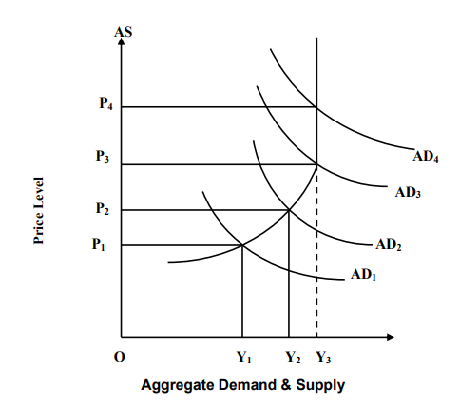
Demand pull inflation is depicted in the above. It is observed that aggregate demand and supply curves are measured along the X-axis and the general price level is measured along the Y-axis. The aggregate supply curve AS rises upward in the beginning and becomes vertical when full employment level of output is achieved at point OYf. This is because the supply of output cannot be increased once full employment level of output is achieved. When the aggregate demand curve is AD1, the equilibrium is less than full employment level and the price level OP1 is determined. When aggregate demand increases to AD2, the price level rises to OP2 due to excess demand at price level OP1. Since the economy is operating at less than full employment level, the real sector of the economy responds to rise in prices and hence the output increases to OY2. When the aggregate demand further rises to AD3, the price level rises to OP3 followed by increase in output to OYf. When the aggregate demand further rises to AD4, the aggregate supply does not respond to remain constant at OYf and only the price level rises to OP4. After the full employment level of output the aggregate supply curve becomes perfectly inelastic and parallel to the Y-axis.
Causes of demand pull inflation-
2. Expectation of inflation – Once people expect inflation in future, they tend to buy more to avoid higher prices. This leads to increase in demand and creates demand-pull inflation. It’s difficult to eradicate once the expectation of inflation sets in.
3. Over expansion of the money supply – This happens when too much money chasing too few goods. An expansion of the money supply with too few goods to buy makes prices increase.
4. Discretionary fiscal policy - According to Keynesian economic theory, government spending drives up demand. Demand increases when government lowers taxes. When consumers have more discretionary income to spend on goods and services it creates inflation.
5. Strong brand - Marketing can create high demand for certain products, a form of asset inflation. This leads to charge high prices
6. Technological innovation – A company owns the market when it creates new technology until other companies figure out how to copy it. People demand new technology that creates real improvement in their daily lives.
Cost push inflation
Cost-push inflation occurs when supply costs rise or supply levels fall. As long as demand remains the same either will drive up prices. Cost push inflation is created by Shortages or cost increases in labor, raw materials, and capital goods.
Definition
Cost-push inflation occurs when firms respond to rising costs by increasing prices in order to protect their profit margins.
Under costpush inflation, price rise due to rise in the cost of raw materials and wages. Sometimes, some producers or workers may raise the prices of their products above the level which prevails in the market. It has been seen that during recession period aggregate demand decrease than supply then prices should also decrease but it did not happen. The cost-push inflation is caused by monopoly which is created by some monopoly groups of the society. It has been seen in the society that labour unions succeed in their demand for higher wages from the industries. Higher wages leads to increase in prices thus is creates wage push inflation which is a part of cost push inflation. Not only labour unions but monopolistic and oligopolistic also increase their profit margin and increase the prices which is known as profit push inflation. Similarly, there can be supply shock inflation.

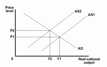
The above diagram shows cost-Push inflation, here AD shows to aggregate demand and AS shows aggregate supply. Is there is increase in AS1 to AS2 then GDP will move from Y1 to Y2 and prices will increase from P1 to P2. This will leads to inflation in the economy. Thus, it can be concluded that cost of factor of production also push inflation in the economy and excess demand is not only a reason for inflation.
Causes of cost push inflation-
2. Wage inflation - Wage inflation is created when workers have enough leverage to force through wage increases. When people expect higher inflation wage may increase in order to protect their real incomes.
3. Component cost – It involves increase in the prices of raw materials and other components. This is due to the rise in commodity prices such as oil, copper and agricultural products used in food processing.
4. Higher indirect taxes – Government regulation and taxation may reduce the supply of many other products such as rise in the duty on alcohol, fuels and cigarettes, or a rise in Value Added Tax.
5. Exchange rates - Higher import prices happens when any country that allows the value of its currency to fall. The foreign supplier does not want the value of its product to drop along with that of the currency. It can raise the price and keep its profit margin intact, if demand is inelastic.
Inflation and interest rate
Inflation refers to the rate at which prices for goods and services rise. In the U.S., the interest rate (which is the amount charged by a lender to a borrower) is based on the federal funds rate that is determined by the Federal Reserve. The Federal Reserve System is the central bank of the U.S.; it is sometimes just referred to as the Fed.
The Fed attempts to influence the rate of inflation by setting and adjusting the target for the federal funds rate. This tool enables the Fed to expand or contract the money supply as needed, which influences target employment rates, stable prices, and stable economic growth.
Under a system of fractional reserve banking, interest rates and inflation tend to be inversely correlated. This relationship forms one of the central tenets of contemporary monetary policy: Central banks manipulate short-term interest rates to affect the rate of inflation in the economy.
Social cost of inflation
An economy which is experiencing inflation has to bear many costs and policymakers, economists and especially politicians are concerned to make arrangements and take steps to curb inflation because of public pressure.
There are different costs of inflation. They are-
Costs of Expected Inflation:
Costs of Unexpected Inflation Unexpected inflation has an effect that is more pernicious than any of the cost discussed under anticipated inflation. It arbitrarily redistributes income and wealth among individuals. We can see how this works by examining long- term loans. Loan agreements specify a nominal interest rate, which is based on the expected rate of inflation
Unanticipated inflation also hurts individuals on pension. Workers and firms often agree on a fixed nominal pension when the workers retire. Since pension is deferred earnings, the workers are essentially providing the firm a loan. Like any creditor, the worker is hurt when inflation is higher than anticipated. Like any debtor, the firm is hurt when inflation is lower than anticipated
Unemployment, also referred to as joblessness, occurs when people are without work and actively seeking employment. Unemployment is very often a characteristics of underdeveloped economie A fast increase in population aggravates the situation by adding a large number of entrants to the labour force every year. In the absence of appreciable rise in industrial investment and with the population growth unchecked, unemployment increases by leaps and bounds.
Definition
In the words of Pigou, “A man is unemployed only when he is both without a job or not employed and also desires to be employed.”
“It is a kind of situation where the unemployed person do not find any meaningful or gainful job inspite of having willingness and capacity to work.”
According to Keynes, “Full employment is a situation in which aggregate employment is inelastic in response to an increase in effective demand for its output.”
Natural rate of unemployment
Natural unemployment, or natural rate of unemployment, is the unemployment rate that persists in a well-functioning, healthy economy that is considered to be at “full employment.” It is a hypothetical rate of unemployment and suggests that there is never zero unemployment in an economy.
Natural unemployment refers to the unemployment that exists when the labor market is in perfect equilibrium.
The theory behind natural unemployment suggests that there is never zero unemployment even in a healthy economy due to the presence of frictional, structural, and cyclical unemployment. When the economy is at the natural rate of unemployment, it is said to be at the “full employment” level and to have reached its potential real GDP.
Components
1. Frictional Unemployment
Frictional unemployment occurs when workers are “in-between jobs,” i.e., when people in the workforce are looking for jobs but are unable to find one yet. It includes recent graduates and employees facing unexpected layoffs that are actively searching. To reduce frictional unemployment, the government must focus its resources on decreasing information costs so that there is a higher amount of job market information present in the economy.
2. Structural Unemployment
Structural unemployment refers to unemployment that is caused due to a mismatch between the skills that a worker offers and those that employers demand. An example of structural unemployment is a scenario where a software engineer is skilled at a coding language that is outdated, which results in unemployment. Offering training programs and subsidized education for skill-building is a way to reduce structural unemployment.
3. Surplus Unemployment
Surplus unemployment is caused by wage rigidity and changes in minimum wage laws. For example, if authorities decide to increase the minimum wage by $2 at any given time, some workers are likely to be laid off due to lowering labor demands. This contributes to natural unemployment in the economy.
Frictional and wait unemployment
Frictional unemployment is the unemployment which exists in an economy due to change in job from one to another. It is the time spent between jobs when a worker is searching a new job or transferring from one to another. It arises a person may be looking for a good job, better opportunities, service or wages due to dissatisfaction with the previous job. Trade union strikes may also create frictional unemployment. One of the kind of frictional unemployment is called wait unemployment.
Definition
“Frictional unemployment is the time period between jobs when a worker is searching for, or transitioning from one job to another. It is sometimes called search unemployment and can be voluntary based on the circumstances of the unemployed individual”
Wait unemployment is the effects of the existence of some sectors where employed workers are paid more than the market clearing equilibrium wage. It arises from wage rigidity and job rationing. The people are unemployed not because they are searching for the jobs but because at the prevailing wage rate supply of labour is greater than the demand for labour. Wait unemployment not only restricts the amount of employment in the high wage sector, but it attracts workers from other sector who wait to try to get jobs there. The main problem is that such workers will likely wait while having jobs, so that they are not counted as unemployed.
Frictional Unemployment is Voluntary
The next point to note about frictional unemployment is that it is voluntary. In the case of frictional unemployment it is the workers who quit their jobs in search of better pursuits. Some of them do find a better job whereas the others have to settle for what they already had. However, it is important to note that the employers are not asking the workers to leave.
This facet is extremely important because involuntary unemployment is associated with a lot of social evils. Employees whose services are no longer required are not prepared to handle the challenge and could face situations as grave as poverty and starvation.
Root Cause of Frictional Unemployment
Frictional unemployment is not caused by a shortage of jobs in the economy. It must be noted that this kind of employment is not a symptom that the number of individuals present in the labor force are more than the number of jobs present in the economy. Rather, frictional unemployment is caused by information mismatch. There is a high probability that both Ms B and worker A will find an employer that suits their needs. They are however not aware as to who that employer is and how to get in touch with them. Therefore, searching the right employer is taking them a while and they are currently being classified as unemployed. If there were a way to improve the information system in the economy, then the amount of frictional unemployment can be drastically reduced. Also, a lot of times, employers wait for an existing employee to quit the job before they take a new one on board. Hence, even if a person has a job which they will start working on at a future date, they will be classified as frictionally unemployed.
Cure for Frictional Unemployment
Most of the developed world is already living in the information age. In countries like UK, US and Germany, the information systems pertaining to jobs are already well developed and frictional unemployment has been drastically reduced. This reduction has been made possible by private job listing sites and placement agencies which keep a database of the jobs and job seekers and match them at the earliest. However, in the developing world, the situation is different. The problem is not grave though and can be simply solved by adopting the same measures that have been adopted by developed countries.
Key takeaways-
In 1958, AW Phillips, a professor at the London School of Economics published a study of wage behavior in the United Kingdom for the years 1861 and 1957. Phillips found an inverse relationship between the rate of unemployment and the rate of inflation or the rate of increase in money wages. The higher the rate of unemployment, the lower the rate of wage inflation i.e. there is a tradeoff between wage inflation and unemployment. The Phillips curve shows that the rate of wage inflation decreases with the increase unemployment rate. Assuming Wt as the wages in the current time period and Wt+1 in the next time period, the rate of wage inflation, gw, is defined as follows:

By representing the natural rate of unemployment with u* , the Phillips curve equation can be written as follows:

where ε measures the responsiveness of wages to unemployment. This equation states that wages are falling when the unemployment rate exceeds the natural rate i.e. when u > u* , and rising when unemployment is below the natural rate. The difference between unemployment and the natural rate, u – u * is called the unemployment gap. Let us assume that the economy is in equilibrium with stable prices and the level of unemployment is at the natural rate. At this point, if the money supply increases by ten per cent, the wages and the price level must rise by ten per cent to enable the economy to be in equilibrium. However, the Phillips curve shows that for wages to rise by ten per cent, the unemployment rate will have to fall. A fall in the unemployment rate below the natural level will lead to increase in wage rates and prices and the economy will ultimately return to the full employment level of output and unemployment. This situation can be algebraically stated by rewriting equation one above as follows.

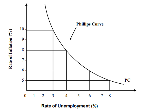
Thus for wages to rise above their previous level, unemployment must fall below the natural rate. The Phillips curve relates the rate of increase of wages or wage inflation to unemployment as denoted by equation two above, the term ‘Phillips curve’ over a period of time came to be used to describe a curve relating the rate of inflation to the unemployment rate. Such a Phillips curve is depicted in Fig.
Its observed that when the rate of inflation is ten per cent, the unemployment rate is three per cent and when the rate of inflation is five per cent, the rate of unemployment increases to eight per cent. Empirical or objective data collected from other developed countries also proved the existence of Phillips Curve. Economists believed that there existed a stable Philips Curve depicting a tradeoff between unemployment and inflation. This trade-off presented a dilemma to policy makers. The dilemma was a choice between two evils, namely: unemployment and inflation. In a dilemma, you chose a lesser evil and inflation is definitely a lesser evil for policy makers. A little more inflation can always be traded off for a little more employment. However, further empirical data obtained in the 70s and early 80s proved the non-existence of Phillips Curve. During this period, both Britain and the USA experienced simultaneous existence of high inflation and high unemployment. While prices rose rapidly, the economy contracted along with more and more unemployment.

Keynesian explanation of Philips curve
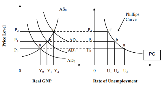
The explanation of Phillips curve by the Keynesian economists is shown in the below Fig. Keynesian economists assume the upward sloping aggregate supply curve. The AS curve slopes upwardly due to two reasons. Firstly, as output is increased in the economy, the law of diminishing marginal returns begins to operate and the marginal physical product of labor (MPPL) begins to decline. Since the money wages are fixed, a fall in the MPPL leads to a rise in the marginal cost of production because MC = W/ MPPL. Secondly, the marginal cost goes up due a rise in the wage rate as employment and output are increased. Following rise in aggregate demand, demand for labor increases and hence the wage rate also increases. As more and more labor is employed, the wage rate continues to rise and the marginal cost of firms increases. You may notice that in Panel (a) of the below fig that with the initial aggregate demand curve AD0 and the given aggregate supply curve AS0, the price level P0 and output level Y0 are determined. When the aggregate demand increases, the AD0 curve shifts to the right and the new aggregate demand curve AD1 intersects the aggregate supply curve at point ‘b’. Accordingly, a higher price level P1 is determined along with a rise in GNP to Y1 level. With the increase in the real GNP, the rate of unemployment falls to U2. Thus the rise in the price level or the inflation rate from P0 to P1, the unemployment rate falls down thereby depicting an inverse relationship between the price level and the unemployment rate. Now when the aggregate demand further increases, the AD curve shifts to the right to become AD2. The new aggregate demand curve AD2 intersects the aggregate supply curve at point ‘c’. Accordingly, the price level P2 and output level Y2 is determined. The level of unemployment now falls to U3. In Panel (b) of the figure, points a, b and c are plotted and these points corresponds to the three equilibrium points a, b and c in Panel (a) of the figure. Thus a higher rate of increase in aggregate demand and a higher rate of rise in price level are related with the lower rate of unemployment and vice versa. The Keynesian economists were thus able to explain the downward sloping Philips curve showing inverse relation between rates of inflation and unemployment.

Key takeaways –
Sources
1. Ahuja H.L – Macro Economics – S.Chand.
2. Mankiw, N. Gregory. Principles Macroeconomics.Cengage Learning.
3. Dornbusch, Rudiger, and Stanley. Fischer, Macroeconomics. McGraw-Hill.
4. Dornbusch, Rudiger., Stanley. Fischer and Richard Startz, Macroeconomics. Irwin/McGraw-Hill.
5. Deepashree, Macro Economics, Scholar Tech. New Delhi.
6. Barro, Robert, J. Macroeconomics, MIT Press, Cambridge MA.