UNIT 5

Linear Programming

5.1 Formulation of linear programming problems (LPP): Graphical solution to LPPs. Cases of unique and multiple optimal solutions, Unbounded solutions and infeasibility, and redundant constraints, Solution to LPPs using Simplex method – maximization and minimization cases.

We use linear programming to optimize the linear function subject to given linear constraints.

LPP is the popular mathematical technique which is used to make maximum profit and minimum loss.

Important definitions-

Linear programming problem-

We need to optimize the linear function Z subject to certain conditions, these types of problems are called Linear programming problem or in short LPP.

Objective functions-

This is a linear function of several variables, subject to the conditions.

Optimal value-

This is a maximum or minimum value of a object function which is to be calculated in a LPP.

Formulation of LPP-

Let’s consider the following example-

Example: A manufacturer produces two types of products ‘P’ and ‘Q’. Each ‘P’ type of product required 4 hours of grinding and 2 hrs of polishing, where ‘Q’ product requires 2 hrs of grinding and 5hrs of polishing.

The manufacturer has 2 grinders and 3 polishers. Each grinder works for 80hrs a week and each polisher works for 180hrs a week. Profit on ‘P’ product is Rs. 3 and profit on ‘Q’ is Rs. 4.Whatever is produced in a week is sold in the market.

How should the manufacturer allocate his capacity of production of two types of products so that he may make the maximum profit and minimum loss in a week?

Now we formulate this problem in mathematical terms as explained below-

Suppose is the number of ‘P’ product and is the number of ‘Q’ product produced weekly.

Then the weekly profit is-

Here ‘Z’ is called the objective function which is to be maximize or minimize.

Now, to produce these number of products, the total number of grinding hours needed weekly is-

And the total number of polishing hours needed per week is-

Here the number of grinding hours is not more than 80 and the number of polishing hours is not more than 180, so that we write,

This is called the first constraint]

[This is the second constraint]

Since the number of product is non-negative, then we can write-

This is called the third constraint.

Hence we form the problem mathematically as follows-

To maximize-
 

Subject to the constraints:

This expression is called as mathematical formulation.

Note- The variables that enter into the problem are called ‘decision variables’.

Example: A dietician mixes together two kinds of food, say, A and B in such a way that the mixture contains at least 6 units of vitamin P, 7 units of vitamin Q, 12 units of vitamin R and 9 units of vitamin S. The vitamin contents of 1 kg of food A and 1 kg of food B are given below:

One kg of food X costs Rs. 5, whereas one kg of food Y costs Rs. 8. Formulate the linear programming problem.

Sol.

Decision variables- Here decision variables are units of food A and B.

Let food A in the mixture be and food B in the mixture .

Objective function- To minimize the cost,

Total cost of food A and B  =

Or

Now we will write the constraints one by one-

Constraint-1: 

Constraint-2: 

Constraint-3: 

Constraint-4: 

Constraint-5: 

Mathematical formation will be as follows-

To minimize,

Subject to the constraints-

Example: A manufacturer has 3 machines 1, 2 and 3. Machines 1 and 2 are capable of being operated for at the most 12 hours whereas machine 3 must be operated at least for 5 hours a day. He produces two items each requiring the use of the three machines.

The number of hours required for producing 1 unit of each of the items X and Y on the three machines are given below:

She makes a profit of Rs. 60 on item X and Rs. 40 on item Y. Assuming that he can sell all that he produces, how many of each item should be produced so as to maximize the profit. Formulate the above as L.P.P.

Sol.

Decision variables- Here decision variables are item X and Y.

Let the production of item X be and the production of item Y be .

Objective function- To maximize the profit,

Now we will write the constraints one by one-

Constraint-1: 

Constraint-2: 

Constraint-3: 

Constraint-4: 

Mathematical formation will be as follows-

To maximize,

Subject to the constraints-

Key takeaways-

Graphical method

LPP having two variables can be easily solved by graphical method which provides a pictorial representation of the solution and we get insights into the basic concept used in solve LPP.

Step by step procedure to solve LPP graphically-

Now plot the given constraints on

coordinate plane and find the convex region.

Note- The region satisfying all the constraints is called feasible region.

Example: Solve the following LPP graphically-

Maximize-

Subject to the constraints-

Sol.

Change the given constraints into equations-

The line   meets the x-axis at the point A(10,0) and meets the y-axis at the point B(0,5). Join A and B to get the graph for the line.             

Hence origin (0,0) satisfies the inequality so that half plane containing the origin represent the solution set of .

And

The line meets the x-axis at the point C(5,0) and meets the y-axis at the point D(0,15). Join C and D to get the graph for the line.

Hence origin (0,0) satisfies the inequality   so that half plane containing the origin represent the solution set of.

Now all the points in first quadrant satisfies  .

So that first quadrant is the region represented by

Hence the region OCEBO satisfies all the inequalities.

And each point on the region is the feasible solution of the problem.

Feasible solution-

Here in this problem the feasible solution is (5,0), (4,3) and (0,5).

Now we can obtain the optimal solution of the problem.

As we know that any point in the feasible region that gives the optimal value is called an optimal solution.

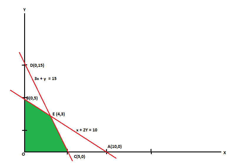
The value of the objective function at corner points of the feasible region is given below-

Here we see that the maximum value of Z is 18.

Note-

Example: Find the maximum value of Z = 2x + 3y subject to the constraints-

Sol.

Any point (x,y) satisfying the conditions lies in the first quadrant only.

Also since the desired point (x,y) lies within the convex region ABCDE.

Its vertices are A(3,3), B(20,3), C(20,10), D(18,12) and E(12,12).

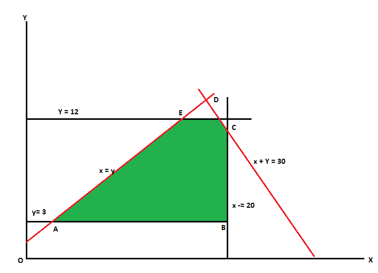
The value of Z at these points are-

Z(A) = 15

Z(B) = 49

Z(C) = 70

Z(D) = 72

Z(E) = 60

Here 72 is the maximum value which is at D.

So that the solution of the LPP is x = 18 and y = 12 and maximum Z  = 72

Example: A factory manufactures two types of items, A and B, each type requiring the use of two machines, an automatic and a hand operated. It takes 4 minutes on the automatic and 6 minutes on hand operated machines to manufacture a package of item A, while it takes 6 minutes on automatic and 3 minutes on the hand operated machines to manufacture a package of item B. Each machine is available for at the most 4 hours on any day. The manufacturer can sell a package of item A at a profit of Rs. 7 and item B at a profit of Rs 10. Assuming that he can sell all the items he manufactures, how many packages of each type should the factory owner produce in a day in order to maximise his profit ?

Determine the maximum profit.

Sol.

We can tabulate the data as follows-

Decision variables- Let the manufacturer produce x packages of item A and y packages of item B per day respectively.

Objective function-  Suppose Z denotes the maximum profit,

Constraints-

1st constraint-

2nd constraint-

3rd constraint-

Mathematical formulation-

The mathematical form of this LPP can be written as-

Maximize
 

Subject to the constraints-

Tables for the region represented by inequalities-

For the first constraint-

For second condition-
 

Now we draw on x and y axes.

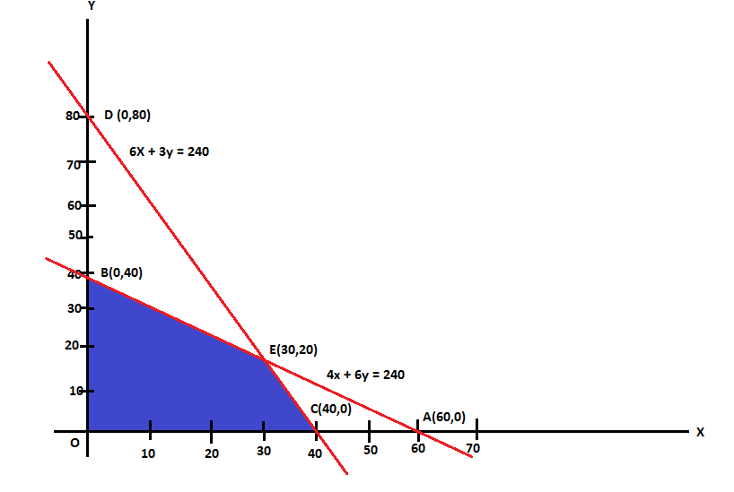
The coordinates of the vertices O, C, E and B of the feasible region OCEBO are O (0, 0), C (40, 0), E (30, 20) and B (0, 40). The coordinates of E are obtained by solving the equations 4x + 6y = 240 and 6x + 3y = 240.             

Therefore Z is maximum at x = 30 and y = 20 and the maximum value of Z is 410.

Special Cases in Linear Programming

a. Infeasible Solution (Infeasibility)

Infeasible means not possible. Infeasible solution happens when the constraints have contradictory nature. It is not possible to find a solution which can satisfy all constraints.

In graphical method, infeasibility happens when we cannot find Feasible region.

Example 1:

Max. Z = 5 X1 + 8 X2

Subject to constraints

4 X1 + 6 X2 ≤ 24

4 X1 + 8 X2 ≤ 40

X1, X2 ≥ 0

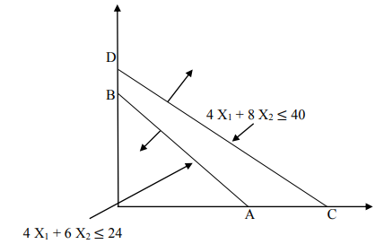
There is no common feasible region for line AB and CD.

Hence, solution is infeasible.

b. Unbounded Solution (Unboundedness)

Unbounded mean infinite solution. A solution which has infinity answer is called unbounded

solution.

In graphical solution, the direction with respect to origin is as follows:

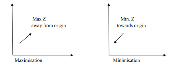
Now, in a maximisation problem, if we have following feasible region:

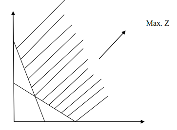
There is no upper limit (away from origin), hence the answer will be infinity. This is called unbounded solution.

c. Redundant Constraint (Redundancy)

A constraint is called redundant when it does not affect the solution. The feasible region does not depend on that constraint.

Even if we remove the constraint from the solution, the optimal answer is not affected.

Example

Max. Z = 5 X1 + 8 X2

Subject to Constraints

3 X1 + 2 X2 ≤ 24

X1 + 3 X2 ≤ 12

X1 ≤ 16

X1, X2 ≥ 0

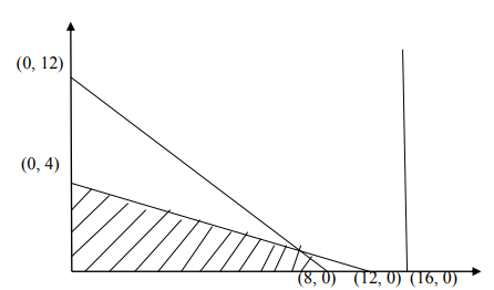
The feasible region for the above problem is OABC. The 3rd constraint does not affect the feasible region.

Hence, the constraint X1 ≤ 16 is redundant constraint.

d. Alternate Optimal Solution: (Multiple Optimal Solution)

Alternate or multiple optimal solution means a problem has more than one solution which gives the optimal answer.

There are two or more sets of solution values which give maximum profit or minimum cost.

In graphical method, we come to know that there is optimal solution which is alternative

when:

The iso-profit or iso-cost line is parallel to one of the boundaries of feasible region (they have the same slope value).

SPECIAL CASES IN SIMPLEX

1. Unbounded Solution

Max Z = 60 X1 + 20X2∆

Subject to

2 X1 + 4X2 ≥ 120

8 X1 + 6X2 ≥ 240

X1, X2 ≥ 0

Solution

Max Z = 60 X1 + 20X2 + 0S1 + 0S2 - MA1 - MA2

Subject to

2 X1 + 4X2 - S1 + A1 = 120

8 X1 + 6X2 - S2 + A1 = 240

X1, X2, S1, S2, A1, A2, ≥ 0

When we solve this LPP by simplex method, we will get the following values in 4th Simplex Table.

Max Positive Cj - Zj = 30

Key Column = S1

But there is no positive Replacement Ration R means there is an Entering variable, but there is no outgoing variable.

Hence, the solution is unbounded or infinity.

The value of Z (Profit) keeps on increasing infinitely.

2. Infeasible Region

Max Z = 3 X1 + 2 X2

Subject to:

X1 + X2 ≤ 4

2 X1 + X2≥ 10

X1, X2 ≥ 0

Solution

Standard Form

Max Z = 3 X1 + 2 X2 + 0S1 + 0S2 - MA1

Subject to

X1 + X2 + S1 = 4

2 X1 + X2 - S2 + A1 = 10

X1, X2, S1, S2, A1 ≥ 0

When we solve this LPP by simplex method, we will get the following values in 2nd Simplex Table.

No positive ∆ value.

All Cj - Zj values are either zero or negative. Hence, test of optimality is satisfied. So, the solution appears to be optimal. But an artificial variable (A1) is present in the basis, which has objective function coefficient of - M (infinity).

Hence, the solution is infeasible (Not feasible).

Infeasibility occurs when there is no solution which satisfies all the constraints of the LPP

References-