UNIT III
Spreadsheet and its Business Applications
You may also use a spreadsheet to create data visualisations, such as maps, to show the statistical data you've gathered on a website.
Spreadsheet Layout:
Creation of Spreadsheet Applications; Range, Formulas, Function:
the fundamentals to making your first Microsoft Excel spreadsheet A spreadsheet is a document with columns and rows of cells for sorting and manipulating data. Each cell is intended to store a single piece of information, such as numbers, letters, or formulas that correspond to other cells. After that, the data can be organised, formatted, graphed, and referred to in other records.
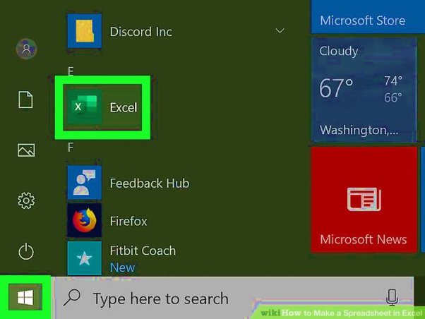
Excel can now be available. It's in the Start menu (Windows) or the Applications folder (Mac) (macOS). You'll be taken to a screen where you can make or pick a folder. If you don't have a premium version of Microsoft Office, you can make a simple spreadsheet using the free online version at https://www.office.com. Everything you have to do now is sign in with your Microsoft account and choose
Excel in the row of icons. 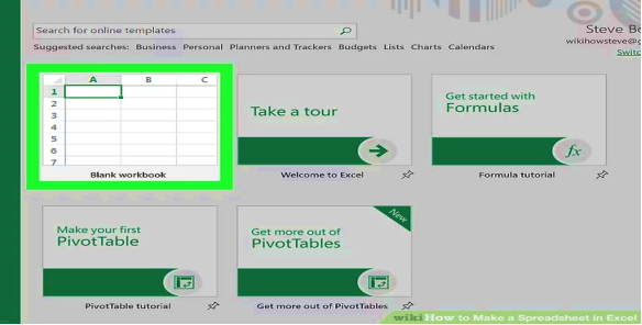
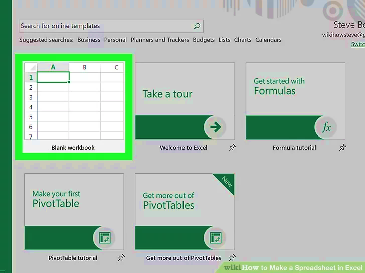
To make a new workbook, click Blank workbook. The name of the folder that includes your spreadsheet is called a workbook (s). This produces Sheet1, a blank spreadsheet that you can access through the tab at the bottom of the sheet. When creating more complicated spreadsheets, press + next to the first sheet to add another line.To swap between spreadsheets, use the bottom tabs.
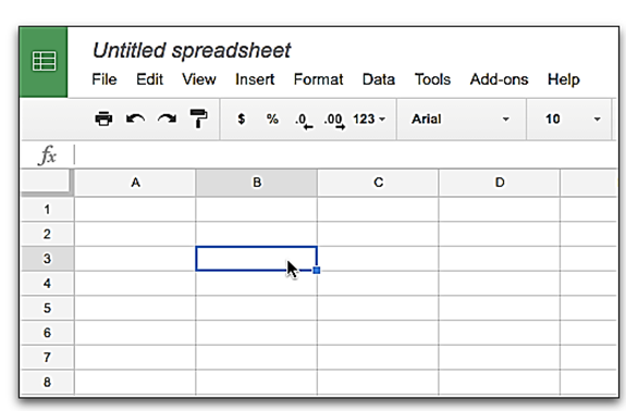
Familiarize yourself with the style of the spreadsheet. The spreadsheet comprises hundreds of rectangular cells divided into vertical columns and horizontal rows, which is the first thing you'll remember. There are a few things to keep in mind about this design:
Along the side of the spreadsheet, all rows are labelled with numbers, while the columns are labelled with letters.
Each cell has a unique address that begins with the column letter and ends with the row number. The address of the cell in the first column (A), first row (1), for example, is A1. The cell in column B row 3 has the address B3.
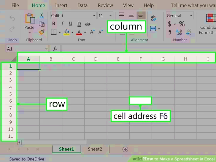
Fill in the blanks. Simply click any cell once and begin typing right away. Click the Tab key to move to the next cell in the list, or the Enter key to move to the next cell in the column, when you're done with that cell.
See how the content of the cell shows in the bar that runs across the top of the spreadsheet when you write. This bar is known as the Formula Bar, and it comes in handy when entering long strings of data or formulas.
Double-click a cell that already has data to pull back the cursor and edit it. You may also press the cell once and change the formula in the formula bar.
To delete data from a single cell, first click it and then press Del. This leaves the cell vacant without affecting the data in adjacent rows or columns. To delete several cell values at once, hold down Ctrl (PC) or Cmd (Mac) while clicking each cell, then press Del.
Right-click the letter above the column after which you'd like the new one to appear, and then select Insert from the context menu.
To insert a new blank row between current rows, right-click the row number for the row after the desired position and choose Insert from the menu.
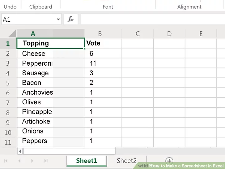
Examine the features that are available for specialised uses. Excel's ability to look up data and make equations based on mathematical formulas is one of its most valuable functions. Each formula you write includes an Excel function, which is the "action" you're carrying out. Formulas often begin with an equal (=) symbol, followed by the function name (for example, =SUM, =LOOKUP, =SIN). Following that, the parameter.
At the top of the page, choose the Formulas tab. In the panel called "Function Library," you'll find some icons in the toolbar at the top of the application. You can quickly search the library using certain icons until you understand how the various functions operate.
The Insert Function button, which also shows a fx, should be clicked. The first icon on the bar should be that. This brings up the Insert Function window.
From the "Or pick a category" menu, choose a category. "Most Recently Used" is the default type. Select Math & Trig, for example, to see the math functions.
In the "Select a function" panel, click any function to see its syntax and a rundown of what it does. Click the Help button for more information on a function.
When you're finished surfing, click Cancel.
See How to Type Formulas in Microsoft Excel for more information on entering formulas.
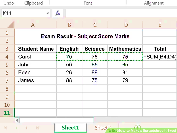
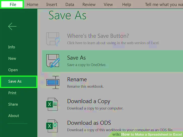
When you're done editing, save your file. To save the file, go to the top-left corner of the screen and pick File > Save As. Depending on the Excel edition, you will be able to save the file to your device or to OneDrive.
Check out the "Creating a Home Inventory from Scratch" approach and see this stuff in action now that you've mastered the fundamentals.
Wherever you save your workbook (such as your computer or the web), save everything on the File tab.
Use Save or press Ctrl + S to save the existing workbook to its current location, but use Save As to save the workbook to another location for the first time. You need to make a copy of the workbook. Same place or different place.
Note: If you are trying to save a macro-enabled workbook (.xlsm) as a regular workbook (.xlsx), be aware that the macro will not be saved in a new file and may lose functionality as a VBA macro. please. It's a powerful way to automate a lot of work. Consider saving the macro or keeping the macro-enabled file until you are sure that the new file has the functionality you expect.
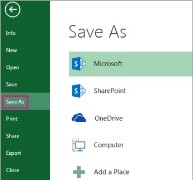
Under Save As, select a location to save your workbook. For example, click Computer to save to a folder on your desktop or computer.
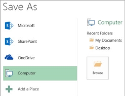
Tip: To save to your OneDrive location, click OneDrive, then sign up (or sign in). Click Add Location to add your own location to the cloud, such as Microsoft 365 SharePoint or OneDrive locations.
Click Browse to find the desired location in the Documents folder.
To choose a different location on your computer, click Desktop, then select the exact location where you want to save your workbook.
In the File name box, type a name for your new workbook. If you want to make a copy of an existing workbook, enter a different name.
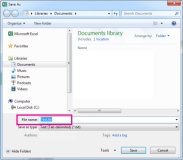
To save the workbook in a different file format (such as .xls or .txt), in the File Types list (under the File Name box), select the format you want.
Click Save.
Secure your favourite storage location
Once you have saved the workbook, you can "pin" the saved location. This makes the location available and can be used again to store another workbook. This can save you time if you tend to save many in the same folder or location. You can fix as many locations as you need.
Click File> Save As.
Under Save As, select the location where you last saved the workbook. For example, if you want to last save the workbook to your computer's Documents folder and pin the location, click Computer.
In Recent Folders on the right, point to the location you want to pin. Pushpin image the pushpin button is displayed on the right.
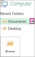
Click the image to pin the folder. The image is displayed as a pinned pushpin icon. Each time you save a workbook, this location will appear at the top of the list under Recent Folders.
Tip: To unlock the location, click the pinned pushpin image again. Fixed push pin icon.
Editing a Workbook
How to edit a worksheet with the help of the Edit Worksheet Steps
Edit the worksheet to vary the design and behavior of the worksheet. For instance, you'll change the layout of worksheet data and add calculations, percentages, or totals.
To edit a worksheet with the help of the Edit Worksheet Steps
On the tabs of the Edit Worksheet dialog, you'll edit the properties of the present worksheet as follows:
See the type tab
Note: the type tab only appears for table worksheets. To sort the crosstab worksheets, select Tools> Worksheets. once you sort, the type Crosstab dialog is displayed (for more information, see the way to Sort Data during a Crosstab Worksheet).
Use the Parameters tab to manage existing parameters and make new ones (see Edit Worksheet Dialog: Parameter Tab for more information).
Click okay to save your changes and return to the worksheet.
Discoverer updates the worksheet with the changes you specify.
Note
You can also edit worksheets directly within the Discoverer workspace using drag-and-drop, right-click menus, and toolbars (see About Discoverer Plus Relational Workspaces for more information).
How to add items to a worksheet
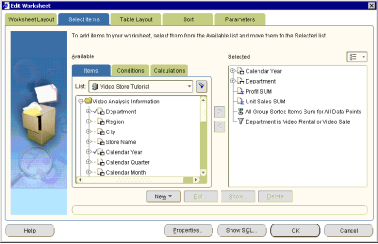
If you would like to use items within the business area to research new areas of your data, add the things to your worksheet. For instance, you would possibly want to feature an item called Year to research trends over time.
For more information on creating new worksheet items (such as calculations and percentages), see the way to Create New Worksheet Items.
Tip: Click the plus (+) sign next to a folder and item to ascertain the things and values in it. Click the flashlight button above the Available box to display the Search Dialog (in Item Navigator) where you'll look for items.
Tip: To reposition worksheet items, attend the Edit Worksheet dialog: Table Layout tab or the Edit Worksheet dialog: Crosstab Layout tab and drag and drop the item. And place it on the worksheet.
Note
To quickly add a worksheet item, simply drag and drop the item from the Available Items pane into the worksheet area. To display the Available Items pane, select View> Items. Available item pane. For more information, see About dragging and dropping items within the Discoverer workspace.
To move an item from the Available list to the chosen list, do one among the following:
How to create a replacement worksheet item
Create a replacement worksheet item if you would like to research different data with items which will not be in your business area. For instance, you'll want to make a three-month mobile sales average.
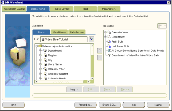
For more information on the way to add an existing item to a worksheet, see the way to Add an Item to a Worksheet.
Note:
To quickly create a replacement worksheet item, select the item within the Selected Items pane and click on one among the following:
Add Item button (e.g., Add Calculation button, Add Percentage button). For more information, see About dragging and dropping items within the Discoverer workspace.
How to remove an item from a worksheet
When you not got to analyze the item, delete it from the worksheet. For instance, you'll delete a year item once you not got to analyze the info over time.
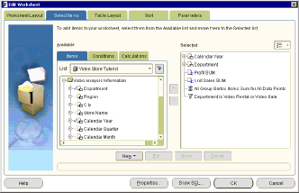
To remove an item from the worksheet:
Note
To quickly delete a worksheet item, right-click the item and select Delete. For more information, see About dragging and dropping items in the Discoverer workspace.
Inserting and deleting worksheets in Excel-Procedures
In this tutorial, you'll study inserting and deleting worksheets in Excel. Inserting and deleting worksheets in Excel is a crucial skill you've got when working with Microsoft Excel workbooks.
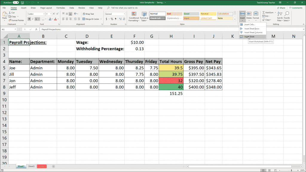
To insert a replacement worksheet to the proper of the currently selected worksheet, click the New Sheet button on the far right of the Spreadsheet Name tab. Alternatively, you'll click the Insert drop-down button within the Cell button group on the house tab of the ribbon. Then select the Insert Sheet command from the menu. Alternatively, you'll press the "Shift" + "F11" keyboard shortcut on your keyboard to automatically insert a replacement worksheet. However, remember that if you employ these last two methods, Excel will insert a replacement worksheet to the left of the active worksheet. this is often a worksheet whose name tab is displayed in bold in color when the sheet is inserted.
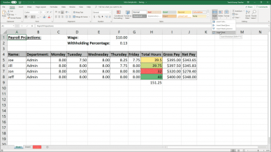
You can reduce the clutter of workbook worksheets by deleting old worksheets that you simply not use. To delete a worksheet in Excel, select the sheet or the worksheet name tab of the sheet you would like to delete. Then click the Delete button within the Cell button group on the house tab of the ribbon. Then click the Delete Sheet command within the button's menu to delete the chosen worksheet.
Inserting and deleting worksheets in Excel: Steps
Manually enter data into worksheet cells
If you want to enter the data manually in Excel, you have several options. You can enter data in one cell, in multiple cells at the same time, or in multiple worksheets at once. The data you enter can be numbers, text, dates, or time. You can format your data in a variety of ways. There are also some settings that you can adjust to make data entry easier.
This topic does not explain how to use data forms to enter data in worksheets. For more information on working with data forms, see Adding, Editing, Finding, and Deleting Rows Using Data Forms.
Important: If you cannot enter or edit data in a worksheet, it may be protected by you or someone else to prevent accidental changes to the data. Protected worksheets allow you to select cells to view data, but you cannot enter information in locked cells. In most cases, do not remove protection from a worksheet without the permission of the worksheet author. To unprotect a worksheet, on the Review tab, in the Changes group, click Unprotect Sheet. If a password was set when worksheet protection was applied, you must first enter that password to unprotect the worksheet.
For example, if you type 3 in the Location box and 2834 in the cell, the value is displayed as 2.834. If you type -3 in the Location box and then 283, the value is 283000.
Enter the date or time as follows:
Tab scroll button
Note: If you don't see the tab for the worksheet you want, click the tab scroll button to find the worksheet and click that tab. If you still can't find the worksheet tab you need, you need to maximize the document window.
Adjust worksheet settings and cell format
Excel has several settings that you simply can change to form it easier to enter data manually. Some changes affect all workbooks, some affect the whole worksheet, and a few affect only specified cells.
Change the direction of the Enter key
If you press Tab to enter data in multiple cells during a row then press Enter at the top of that row, by default the choice moves to the start of subsequent row.
Press Enter to maneuver the choice down one cell, and press Tab to maneuver the choice one cell to the proper. you can't change the direction of the tab , but you'll specify a special direction for the Enter key. Changing this setting affects the whole worksheet, other open worksheets, other open workbooks, and every one new workbook.
On the File tab, click Options.
For Excel 2007 only: Click the image of the Microsoft Office Button , then click Excel Options.
In the Advanced category, under Editing Options, select the Move selection after pressing Enter check box, then click the specified direction within the Direction box.
Change column width
You may see ##### within the cell. this will happen if the cell contains variety or date and therefore the width of that column cannot display all the characters required therein format. For instance, suppose a cell with the date format "mm / dd / yyyy" contains New Year's Eve , 2015. However, the width of the column is sufficient to display 6 characters. ##### is displayed within the cell. you would like to extend the width of the columns to ascertain the whole contents of the cell in its current format.

Note: rather than widening a column, you'll also change the format of that column and therefore the individual cells. for instance , you'll change the format of dates in order that dates are displayed only in months and days ("mm / dd" format), like 12/31, or numbers in scientific (exponential) format, such as: are often represented. 4E +08.
Wrap text in cells
You can display multiple lines of text during a cell by wrapping the text. Wrapping text during a cell doesn't affect other cells.

Click the cell that wraps the text.
On the house tab, within the Alignment group, click Wrap Text.
Placement group on the house tab
Note: For words with long text, the characters aren't wrapped (words aren't split). Instead, you'll widen the columns or reduce the font size to ascertain all the text. If you do not see all the text after wrapping the text, you'll got to adjust the road height. On the house tab, within the Cell group, click Format, and under Cell Size, click Auto Adjust Rows.
Change the format of numbers
In Excel, the cell format is different from the info stored within the cell. This difference in display can have a big impact when the info is numeric. for instance , if the amount you enter is rounded, normally only the displayed number is rounded. The calculation uses the particular number stored within the cell, not the formatted number displayed. Therefore, the calculation may appear inaccurate because one or more cells are rounded.
After entering numbers within the cells, you'll change the format during which they're displayed.
Click the cell that contains the amount you would like to format.
On the house tab, within the Number group, click the arrow next to the amount Format box, then click the format you would like.
Number Format box on the house tab

To select variety format from the list of obtainable formats, click Other Number Formats, then click the format you would like to use within the Categories list.
Format numbers as text
For numbers that ought to not be calculated in Excel, like phone numbers, you'll format them as text by applying the text format to empty cells before entering the amount.
Select an empty cell.
On the house tab, within the Number group, click the arrow next to the amount Format box, then click Text.
Change applies to all selected worksheets.

2. To cancel the selection of multiple worksheets, click on the unselected worksheet. If you don't see a worksheet that isn't selected, right-click the tab for the selected worksheet and click Ungroup Spreadsheet.
3. When you enter or edit data, the changes affect all selected worksheets and can inadvertently replace data that you do not intend to change. To avoid this, you can view all worksheets at the same time to identify potential data races.
Formula Copying, Moving data from selected cells
Windows
It's important to understand how relative cell references can change once you move or copy a formula.
Move Formula: Moving a formula doesn't change the cell references within the formula, no matter the sort of cell reference you employ.
Copy Formula: Copying a formula changes the relative cell reference.
Move formula
This table summarizes how the reference type is updated if the formula containing the reference is copied two cells down and two cells to the proper.

If the reference is: | It changes to: | |
| $A$1 (absolute column and absolute row) | $A$1 |
| A$1 (relative column and absolute row) | C$1 |
| $A1 (absolute column and relative row) | $A3 |
| A1 (relative column and relative row) | C3 |
Note: Fill handle you'll also use the fill handle  to repeat a formula to an adjacent cell. After verifying that the cell reference within the formula produces the result you would like in step 4, select the cell that contains the copied formula and drag the fill handle to the world you would like to fill.
Rearranging Worksheet
How to regroup the text in an Excel cell?
Suppose you've a spreadsheet with long list names, beat the form "Last name First name", and you'd wish to relocate all the names to "First name, Last name". the thanks to achieve that? During this text, I'll show you 3 ways to help you solve your problem.
Sort text in cells using formulas
The following formulas are useful for reversing cell names and names in Excel. Please do as follows.
=TRIM (MID (b2, SEARCH (" “, b2) +1,250)) &" "&LEFT (b2, SEARCH (" “, b2)-1)

Note: within the formula, B2 is that the cell that contains the name you'd wish to relocate. Change it if necessary.
2. Still select the result cell and drag the fill handle right down to flip all the names, as shown within the screenshot below.
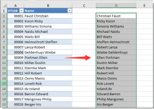
Easily rearrange the text in Excel cells.
Kutools for Excel's Text Inversion Utility allows you to easily swap text within a cell using specific Excel delimiters. See the screenshot below.
Rearrange text in cells using VBA code
In addition, you'll apply the next VBA code to invert all the names within the list directly in Excel. Please do as follows.
1. In order to open the Microsoft Visual Basic for Applications window we need to Press Alt + F11
2. within the Microsoft Visual Basic for Applications window, click Insert> Module. Then copy the next VAB code into the module window.
VBA code: Rearrange text in a cell
1 2 3 4 5 6 7 8 9 10 11 12 13 14 15 16 17
| Sub RearrangeText() 'Updated by Extendoffice 20180503 Dim xRg As Range, yRg As Range Dim LastRow As Long, i As Long Dim strTxt As String, strFs As String Dim strLs As String, N As Integer On Error Resume Next Set xRg = Application.InputBox(Prompt:="Range Selection:", _ Title:="Kutools for excel", Type:=8) For Each yRg In xRg On Error Resume Next strTxt = yRg.Value Trim (strTxt) N = InStr(strTxt, " ") strLs = Left(strTxt, N - 1) strFs = Right(strTxt, Len(strTxt) - N) yRg.Value = strFs & " " & strLs Next End Sub |
3. Next, the Kutools for Excel panel is displayed. Select the name list you'd wish to relocate and click on the OK button. See screenshot:
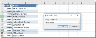
All "first and last names" within the chosen list are immediately flipped.
Quickly rearrange text in cells using Kutools for Excel
This section introduces Kutools for Excel's Reverse Text Ordering Utility to help you rearrange the text in cells.
Before using Kutools for Excel, we need to download and install it first.

2. within the Invert Text panel, select the Space option and click on on the OK button. See screenshot:

Then all the names within the chosen list are getting to be rearranged directly.
Project involving multiple spreadsheets, Organizing Charts and graphs
How do I create a graph between multiple worksheets / from multiple worksheets in Excel?
For example, four worksheets have four tables with the same layout, as shown in the screenshot below. Next, you need to extract the data series from each worksheet to create a graph, and extract the data points from each worksheet to create a graph. How can I solve them in Excel? This article recommends two workarounds:
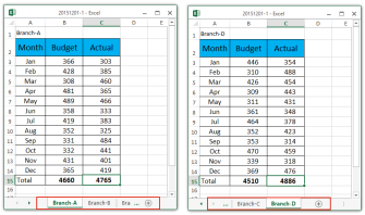
Extract many data series from multiple worksheets to create a graph
This section describes how to extract many data series from multiple Excel worksheets to create a column chart. You can archive by following the steps below.
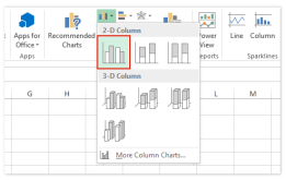
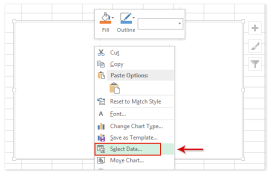
2. Insert a blank chart here. Right-click on the blank graph and select Data from the right-click menu. See screenshot:
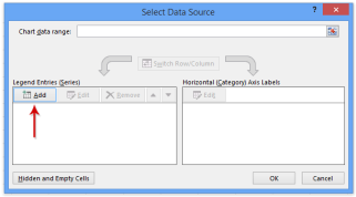
3. Open the Select Data Source dialog box and click the Add button.
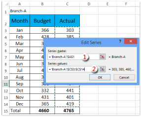
4. In the Edit Series dialog box, specify the series name and series value from the worksheet and click the OK button.
5. When you return to the Select Data Source dialog box, repeat steps 3 and 4 to add data series from other worksheets. Finally, all the data series added from the worksheet are listed in the Legend Entry (Series) box, as shown in the screenshot below.
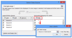
6. In the Select Data Source dialog box, click the Edit button in the Horizontal (Category) Axis Labels section to open the Axis Labels dialog box and specify the axis labels as needed. Click the [OK] button. See the screenshot above.
7. Click the OK button to close the Select Data Source dialog box
8. Optional. Continue to select the graph, click Design> Add Graph Element> Legend, and select Legend Options from the submenu. See screenshot:
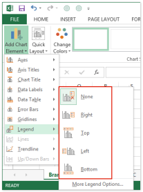
In this example, select Legend> Below.
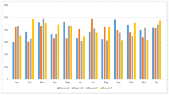
So far, you've created a clustered column chart with four data series from four worksheets. See screenshot:
Extract many data points from multiple worksheets to create a graph
You may want to create a graph whose data points are from different worksheets. This section introduces Kutools for Excel's Dynamically Browse Worksheets to extract data points from multiple worksheets into new worksheets and use these data points to create graphs.
Kutools for Excel-Includes over 300 handy tools for Excel. 30-day full-featured free trial, no credit card required! Free trial now!
1. On the Sheet tab bar, click the New button or create a new worksheet.
2. In the new worksheet, select the cell whose contents you want to extract from other worksheets and click Kutools> Other (in the Formula group)> Dynamic.
See worksheet. See screenshot:
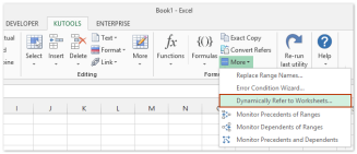
The document dynamically references Sheet 1
3. Open the Enter Worksheet Reference dialog box and do the following:
(1) Select [Fill vertically after cell] from the [Fill order] drop-down list.
(2) In the Worksheet List section, review the worksheet from which you want to extract the data points.
(3) Click the [Fill Range] button and the [Close] button in succession.
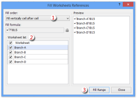
Note: If you have multiple data series with data points from different worksheets, you can repeat this step if necessary.
Then you can see that the data points are extracted from various worksheets. See screenshot:
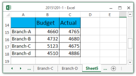
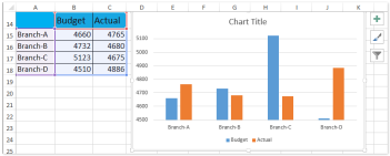
4. Select the extracted data points and create a graph. In this example, click Insert> Insert Column Chart (or Column)> Clustered Columns to create a clustered column.
So far, you've created a clustered column chart with data points from different worksheets. See screenshot:
Print a worksheet
To print a worksheet in Excel, do the following:
1. On the File tab, click Print.
2. To preview the opposite pages which will be printed, click Next Page or Previous Page at rock bottom of the window.
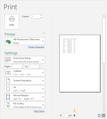
Click the massive Print button to print the worksheet.
Click the large print button

What to Print?
Instead of printing the whole worksheet, you'll also print the present selection.
1. First, select the range of cells to print.
2. Then, under Settings, select Print Selection.
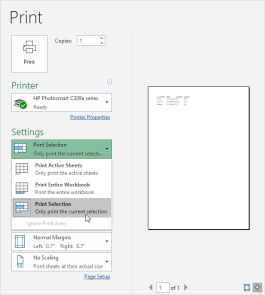
3. Click the massive Print button to print the choice.

Click the large Print button
Note: you'll print the active sheet (CTRL + first click the Sheet tab to pick a sheet), otherwise you can print the whole workbook. Use the box next to Pages (see the primary screenshot) to print only a couple of pages of your document. for instance, 2-2 prints only the second page.
Multiple copies
To print multiple copies, follow these steps:
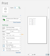
1. Use the arrow next to the Copy box.
2. If a replica contains multiple pages, you'll switch between matched and unmatched. For instance, if you would like to print 6 copies, Collated prints the whole first copy, then the whole second copy. Uncollated prints 6 copies on 1 page, 6 copies on 2 pages, and so on.
Orientation
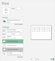
You can switch between portrait orientation (more rows but fewer columns) and landscape orientation (more columns but fewer rows).
Page margin
To adjust the page margins, follow these steps:
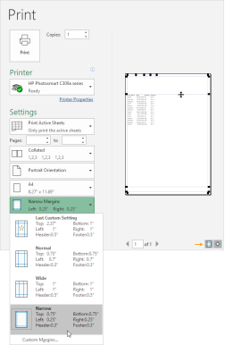
1. From the Margin drop-down list, select one among the predefined margins (Standard, Wide, or Narrow).
2. Alternatively, click the Show Margins icon at rock bottom right of the window. you'll now manually change the page margins by dragging the lines.
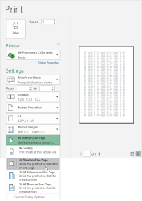
Scaling
If you would like to suit more data on one page, you'll fit the sheet on one page. to realize this, do the following:
Generally used Spread sheet functions:
Excel math functions
Excel has many basic and advanced functions for performing math operations and calculating exponents, logarithms, factorials, and more. It takes a few pages just to publish the function list. So let's discuss only a few basic math functions that may help you solve your daily work.
Find the cell total
Here are four important Excel functions for summing the values in a specified range of cells:
SUM function
SUM (number1, [number2],…) returns the sum of its arguments. The argument can be a number, a cell reference, or a formula-driven number.
For example, the simplest formula = SUM (A1: A3, 1) sums the values in cells A1, A2, and A3, and then adds 1 to the result.
Example of SUM expression:
Both functions sum a specified range of cells that meet certain conditions. The difference is that SUMIFS can only evaluate a single criterion, while SUMIFS introduced in Excel 2007 allows multiple criteria. Note that the order of the arguments is different for each function.
SUMIF(range, criteria, [sum_range]) SUMIFS(sum_range, criteria_range1, criteria1, [criteria_range2, criteria2], …)
The following screenshot shows how the SUMIF and SUMIFS functions can be used with real data.

Examples of SUMIF and SUMIFS expressions
Sum product Function
SUMPRODUCT (array1, array2, ...) is one among the few Microsoft Excel functions to figure with arrays. Multiplies the provided array components and returns the sum of the products.
It is often difficult to know the essence of the SUMPRODUCT function, but I hope the subsequent example sheds light on its main use.
Example of SUMPRODUCT expression:
RAND () Returns a random real (decimal number) from -0 to 1.
RANDBETWEEN (bottom, top)-Returns a random integer between the required bottom and top numbers.
The following tutorials are very helpful in explaining the gist of every function using mathematical formula examples. the way to use the RAND and RANDBETWEEN functions in Excel.
Rounding function
Excel features a sort of functions for rounding numbers, and therefore the Excel Rounding Tutorial explains the way to use these functions supported criteria. Click the name of the function to ascertain its syntax and usage examples.
This function is extremely useful in many scenarios, such as:
Statistical functions in Excel
SUMPRODUCT (array1, array2, ...) is one among the few Microsoft Excel functions to figure with arrays. Multiplies the provided array components and returns the sum of the products.
It is often difficult to know the essence of the SUMPRODUCT function, but I hope the subsequent example sheds light on its main use.
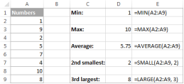
Example of SUMPRODUCT expression:
VLOOKUP SUMPRODUCT expression that's case sensitive
Count duplicates between two columns
Sum cells by multiple criteria
Random number generation (RAND and RANDBETWEEN)
Microsoft Excel provides two functions for generating random numbers. Both are volatile functions. That is, whenever the worksheet calculates s, a replacement number is returned.
RAND () Returns a random real (decimal number) from -0 to 1.
RANDBETWEEN (bottom, top)-Returns a random integer between the required bottom and top numbers.
The following tutorials are very helpful in explaining the gist of every function using mathematical formula examples. the way to use the RAND and RANDBETWEEN functions in Excel.
Rounding function
Excel features a sort of functions for rounding numbers, and therefore the Excel Rounding Tutorial explains the way to use these functions supported criteria. Click the name of the function to ascertain its syntax and usage examples.
Financial Function
Microsoft Excel offers a number of features to simplify the work of accounting managers, financial analysts, and banking specialists. So far, this blog has only described one financial function that can be used to calculate compound interest.
Logical Function
Microsoft Excel provides a small number of logical functions that evaluate a given condition and return the corresponding value.
AND, OR, XOR functions
AND (logical1, [logical2],…)-Returns TRUE if all arguments evaluate to TRUE, FALSE otherwise.
Microsoft Excel provides a small number of logical functions that evaluate a given condition and return the corresponding value.
AND, OR, XOR functions
AND (logical1, [logical2],…)-Returns TRUE if all arguments evaluate to TRUE, FALSE otherwise.
OR (logical1, [logical2],…)-Returns TRUE if at least one of the arguments is TRUE.
XOR (logical1, [logical2],…)-Returns the exclusive OR of all arguments. This function was introduced in Excel 2013 and is not available in earlier versions.
Excel logical functions-AND, OR, XOR.
Example of a logical function expression:
XOR (logical1, [logical2],…)-Returns the exclusive OR of all arguments. This function was introduced in Excel 2013 and is not available in earlier versions.
Excel logical functions-AND, OR, XOR
Date and Time Function
For anyone who works with Excel dates on a daily basis, we recommend a comprehensive 12-part Excel Dates tutorial that details each date function. This page only contains an inventory of features and links to other resources.
Date creation
Calculate working days
Excel time function
Below may be a list of the main Excel functions that employment in time.
Lookup and reference Function
These MS Excel functions are useful once you got to find specific information during a table supported the worth of one column, or once you got to return a regard to a selected cell.
VLOOKUP function
The VLOOKUP function looks up the worth laid out in the primary column and pulls matching data from an equivalent row in another column. you would like the subsequent arguments:
VLOOKUP (lookup_value, table_array, col_index_num, [range_lookup])
lookup_value-The value to seem up.
table_array-2 columns or more of knowledge.
col_index_num-The number of the column to tug the info from.
range_lookup-Determines whether to look by exact match (FALSE) or approximate match (TRUE or omitted).
For example, the formula = VLOOKUP ("apples", A2: C10, 3) searches for "apples" in cells A2 through A10 and returns matching values from column C.
Example of VLOOKUP expression:
Excel VLOOKUP tutorial for beginners
How to work with VLOOKUP & SUM or SUMIF functions in Excel
Bidirectional lookup, nested VLOOKUP with multiple criteria
4 Ways to Perform a Case Sensitive VLOOKUP in Excel
Excel VLOOKUP doesn't work-Solution for N / A, NAME, and VALUE errors.
INDEX function
INDEX (array, row_num, [column_num])-Returns a regard to a cell within the array supported the required row and column numbers.
Here may be a simple INDEX formula: = INDEX (A1: C10, 3, 4) searches cells A1 to C10 and returns the worth in cell D3, which is that the intersection of the 3rd and 4th columns.
The following tutorial will take a better check out the INDEX function. The 6 most effective uses of the INDEX function in Excel.
Text Functions
TEXT function
TEXT (value, format_text) is used to convert a number or date to a test string in the specified format. here,
The value is the number that you want to convert to text.
Format_text is the desired format.
The following formula shows how the Excel TEXT function works.
= TEXT (A1, "mm / dd / yyyy")-Converts the date in cell A1 to a text string in traditional US date format such as "01/01/2015" (month / day / year).
= TEXT (A1, "€ #, ## 0.00")-
Example of TEXT expression:
Key takeaways:
References:
