Unit - 3
The Cauchy problem
The Cauchy problem
Let

Where A(x, y), B(x, y) and C(x, y) are functions of x and y and  be the curve in x, y plane.
The problem of finding the solution u(x, y) and the PDE (1) in the neighbourhood of  satisfying the following conditions

On  is called a Cauchy problem and the above two conditions are called Cauchy conditions.
Consider the Cauchy problem in the case of Laplace’s equation

With the following data prescribed on the x-axis,
U(x, 0) = 0
The intital curve is here is the x-axis,
It is easy to verify that
Is the solution of the above problem.
Observe that when n tends to infinity the function  uniformly.
However  does not become small an n tends to infinity for any non-zero y.
So that the solution is not stable.
We will now show that the solution to the Dirichlet’s problem is stable.
Suppose  and
and  are the solutions of


And


Let v = ( , then

By the maximum and minimum principle, the harmonic function v attains its maximum and minimum on B which is nothing but the maximum and minimum of  .
.
Cauchy problem of an infinite string
In the theory of ordinary differential equations, by the initial-value problem we mean the problem of finding the solutions of a given differential equation with the appropriate number of initial conditions prescribed at an initial point. For example, the second-order ordinary differential equation
d2u/dt2 = f(t, u,du/dt)
And the initial conditions
u (t0) = α, (du/dt)(t0) = β,
Constitute an initial-value problem.
An analogous problem can be defined in the case of partial differential equations. Here we shall state the problem involving second-order partial differential equations in two independent variables.
We consider a second-order partial differential equation for the function u in the independent variables x and y, and suppose that this equation can be solved explicitly for uyy, and hence, can be represented in the from
uyy = F (x, y, u, ux,uy,uxx,uxy) . (1)
For some value y = y0, we prescribe the initial values of the unknown function and of the derivative with respect to y
u (x, y0) = f (x), uy (x, y0) = g (x) . (2)
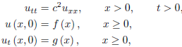
The problem of determining the solution of equation (1) satisfying the initial conditions (2) is known as the initial-value problem. For instance, the initial-value problem of a vibrating string is the problem of finding the solution of the wave equation
utt = c2uxx,
Satisfying the initial conditions
u (x, t0) = u0 (x), ut (x, t0) = v0 (x) ,
Where u0(x) is the initial displacement and v0 (x) is the initial velocity. In initial-value problems, the initial values usually refer to the data assigned at y = y0. It is not essential that these values be given along the line y = y0; they may very well be prescribed along some curve L0 in the xy plane. In such a context, the problem is called the Cauchy problem instead of the initial-value problem, although the two names are actually synonymous.
We consider the Euler equation
Auxx + Buxy + Cuyy = F (x, y, u, ux,uy) , (3)
Where A, B, C are functions of x and y. Let (x0, y0) denote points on a smooth curve L0 in the xy plane. Also let the parametric equations of this curve L0 be
x0 = x0 (λ), y0 = y0 (λ) , (4)
Where λ is a parameter.
We suppose that two functions f (λ) and g (λ) are prescribed along the curve L0. The Cauchy problem is now one of determining the solution u (x, y) of equation (3) in the neighborhood of the curve L0 satisfying
The Cauchy conditions
u = f (λ) , (.5a)
∂u/∂n= g (λ) , (5b)
On the curve L0 where n is the direction of the normal to L0 which lies to the left of L0 in the counter-clockwise direction of increasing arc length.
The function f (λ) and g (λ) are called the Cauchy data.
For every point on L0, the value of u is specified by equation (5a).Thus, the curve L0 represented by equation (4) with the condition (5a) yields a twisted curve L in (x, y, u) space whose projection on the xy plane is the curve L0. Thus, the solution of the Cauchy problem is a surface, called an integral surface, in the (x, y, u) space passing through L and satisfying the condition (5b), which represents a tangent plane to the integral surface along L.
If the function f (λ) is differentiable, then along the curve L0, we have
Du/dλ=(∂u/∂x)(dx/dλ)+(∂u/∂y)(dy/dλ)=(df/dλ) (6)
And
∂u/∂n=(∂u/∂x)(dx/dn)+(∂u/∂y)(dy/dn)= g (7)
But
Dx/dn= −(dy/ds) and dy/dn=dx/ds (8)
Equation (7) may be written as
∂u/∂n= −(∂u/∂x)(dy/ds)+(∂u/∂y)(dx/ds)= g (9)
Since

The equation
A(dy/dx)2 – B(dy/dx)+ C = 0, (10)
Is called the characteristic equation.
Let the partial differential equation be given in the form
uyy = F (y, x1,x2, . . . ,xn,u,uy,ux1,ux2 . . . ,uxn,ux1y,ux2y, . . . ,uxny,ux1x1,ux2x2, . . . ,uxnxn) , (1)
And let the initial conditions
u = f (x1,x2, . . . ,xn) , (2)
uy = g (x1,x2, . . . ,xn) , (3)
Be given on the noncharacteristic manifold y = y0.
If the function F is analytic in some _ neighborhood of the point and if the functions f and g are analytic in some neighborhood of the point
 , then the Cauchy problem has a unique analytic solution in some neighborhood of the point
 .
.
For the proof, see Petrovsky (1954). The preceding statement seems equally applicable to hyperbolic, parabolic, or elliptic equations. However, we shall see that difficulties arise in formulating the Cauchy problem for nonhyperbolic equations. Consider, for instance, the famous Hadamard (1952) example.
The problem consists of the elliptic (or Laplace) equation
uxx + uyy = 0,
And the initial conditions on y = 0
u (x, 0) = 0, uy (x, 0) = n−1 sin nx..
The solution of this problem is
u (x, y) = n−2 sinh ny sin nx,
Which can be easily verified.
It can be seen that, when n tends to infinity, the function n−1 sin nx tends uniformly to zero. But the solution n−2 sinh ny sin nx does not become small, as n increases for any nonzero y. Physically, the solution represents an oscillation with unbounded amplitude(n−2 sinh ny) as y → ∞ for any fixed x. Even if n is a fixed number, this solution is unstable in thesense that u → ∞ as y → ∞ for any fixed x for which sin nx  0. It is obvious then that the solution does not depend continuously on the data. Thus, it is not a properly posed problem. In addition to existence and uniqueness, the question of continuous dependence of the solution on the initial data arises in connection with the Cauchy–Kowalewskaya theorem. It is well known that any continuous function can accurately be approximated by polynomials. We can apply the Cauchy–Kowalewskaya theorem with continuous data by using polynomial approximations only if a small variation in the initial data leads to a small change in the solution.
Homogeneous Wave Equations
To study Cauchy problems for hyperbolic partial differential equations, it is quite natural to begin investigating the simplest and yet most important equation, the one-dimensional wave equation, by the method of characteristics. The essential characteristic of the solution of the general wave equation is preserved in this simplified case.
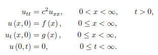
We shall consider the following Cauchy problem of an infinite string with the initial condition
utt − c2uxx = 0, x R, t>0, (1)
u(x, 0) =f(x), x R, (2)
ut (x, 0) = g (x), x R. (3)
The characteristic equation according to equation is
Dx2 − c2dt2 = 0,
Which reduces to
Dx + cdt = 0, dx− cdt = 0.
The integrals are the straight lines
x + ct = c1, x− ct = c2.
Introducing the characteristic coordinates
ξ = x + ct, η = x − ct,
We obtain
uxx = uξξ +2uξη + uηη, utt = c2 (uξξ − 2 uξη + uηη ) .
Substitution of these in equation (1) yields
−4c2uξη = 0.
Since c  0, we have
uξη = 0.
Integrating with respect to ξ, we obtain
uη = ψ∗ (η) ,
Where ψ∗ (η) is an arbitrary function of η. Integrating again with respect to η, we obtain
u (ξ, η) = ψ∗ (η) dη + φ (ξ).
If we set ψ (η) = ψ∗ (η) dη, we have
u (ξ, η) = φ (ξ)+ψ (η),
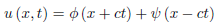
Where φ and ψ are arbitrary functions. Transforming to the original variables x and t, we find the general solution of the wave equation
u (x, t) = φ (x + ct)+ψ (x − ct), (4)
Provided φ and ψ are twice differentiable functions.
Now applying the initial conditions (2) and (3), we obtain
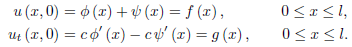
u (x, 0) = f (x) = φ (x)+ψ (x), (5)
Ut (x, 0) = g (x) = cφ′ (x) − cψ′ (x). (6)
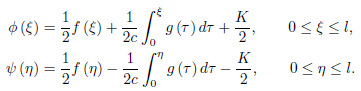
Integration of equation gives
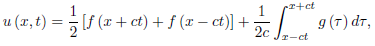
The solution is thus given by
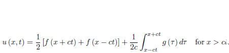
u (x, t) =(1/2)[f (x + ct)+f (x − ct)] +(1/2c)[  g (τ ) dτ −
 g (τ ) dτ]
=(1/2)[f (x + ct)+f (x − ct)] +(1/2c)  g (τ ) dτ. (7)
This is called the celebrated d’Alembert solution of the Cauchy problem for the one-dimensional wave equation.
PDE’s are usually specified through a set of boundary or initial conditions. A boundary condition expresses the behavior of a function on the boundary (border) of its area of definition. An initial condition is like a boundary condition, but then for the time-direction. Not all boundary conditions allow for solutions, but usually the physics suggests what makes sense. Let you remind the situation for ordinary differential equations, one you should all be familiar with, a particle under the influence of a constant force.
 which leads to
 , and
, and
These are linear initial conditions (linear since they only involve xx and its derivatives linearly), which have at most a first derivative in them. This one order difference between boundary condition and equation persists to PDE’s. It is kind of obviously that since the equation already involves that derivative, we can not specify the same derivative in a different equation.
A solution of a PDE in some region R of the space of the independent variables is a function that has all the Partial derivatives appearing in the partial differential equation in some domain D containing R, and satisfies the partial differential equation everywhere in R.
Often one merely requires that the function is continuous on the boundary of R, has doors derivatives in the interior of R, and satisfies the partial differential equation in the interior of R. Letting R lie in D simplifies the situation regarding derivatives on the boundary of R, which is the same on the boundary as it is in the interior of R.
In general, the totality of solutions of a partial differential equation is very large. For example the functions

Which are entirely different from each other, are solutions of (3), as you may verify. We shall see later that the unique solution of a partial differential equation corresponding to a given physical problem will be obtained by the use of additional conditions arising from the problem. For instance this may be the condition that the solution u assume given values on the boundary of the region R (boundary conditions). Or when time t is one of the variables, u may be prescribed at t =0 (initial conditions)
Initial boundary value problem
Semi-infinite String with a Fixed End-
Let us first consider a semi-infinite vibrating string with a fixed end,
That is,
 …..(1)
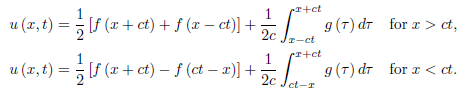
It is evident here that the boundary condition at x = 0 produces a wave moving to the right with the velocity c. Thus, for x > ct, the solution is the same as that of the infinite string, and the displacement is influenced only by the initial data on the interval [x − ct, x + ct],
When x < ct, the interval [x − ct, x + ct] extends onto the negative x-axis where f and g are not prescribed. But from the d’Alembert formula
 …(2)
…(2)
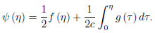
Where
We see that
If we let α = −ct, then
And hence,
The solution of the initial boundary-value problem, therefore, is given by
In order for this solution to exist, f must be twice continuously differentiable and g must be continuously differentiable, and in addition
f (0) = f’’(0) = g (0) = 0.
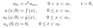
Example: Determine the solution of the initial boundary-value problem
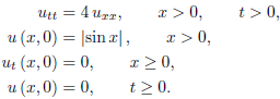
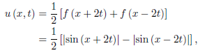
For x > 2t,
And for x < 2t,
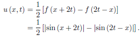
And for x < 2t,

Notice that u (0, t) = 0 is satisfied by u (x, t) for x < 2t (that is, t > 0).
Semi-infinite String with a Free End
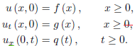
We consider a semi-infinite string with a free end at x = 0. We will determine the solution of
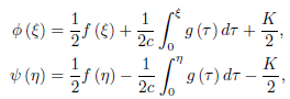
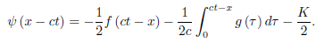
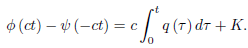
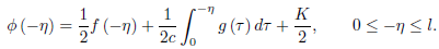
As in the case of the fixed end, for x > ct the solution is the same as that of the infinite string. For x < ct, from the d’Alembert solution

We have

Thus

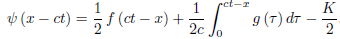
Integration yields
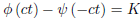
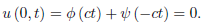
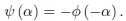
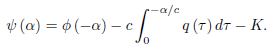
Where K is a constant. Now, if we let α = −ct, we obtain

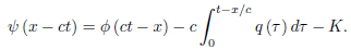
Replacing α by x − ct, we have

And hence,
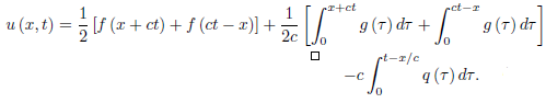
The solution of the initial boundary-value problem, therefore, is given by

For x < ct
We note that for this solution to exist, f must be twice continuously differentiable and g must be continuously differentiable, and in addition,
F’ (0) = g’(0) = 0.
Key takeaways
A solution of a PDE in some region R of the space of the independent variables is a function that has all the Partial derivatives appearing in the partial differential equation in some domain D containing R, and satisfies the partial differential equation everywhere in R.
Equations with Non-homogeneous Boundary Conditions
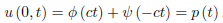
In the case of the initial boundary-value problems with non-homogeneous boundary conditions, such as
u(0, t) = p(t) , 
We proceed in a manner similar to the case of homogeneous boundary conditions.
We apply the boundary condition to obtain
If we let  = −ct, we have
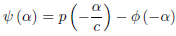
Replacing  by x − ct, the preceding relation becomes
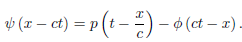
Thus, for 0 ≤ x < ct,

Where 
(x + ct =  ) , and
  (
( ) is given by
In this case, in addition to the differentiability conditions satisfied by f and g, as in the case of the problem with the homogeneous boundary conditions, p must be twice continuously differentiable in t and

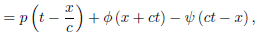
We next consider the initial boundary-value problem

We apply the boundary condition to obtain

Then, by integrating
If we let α = −ct, then
Replacing α by x − ct, we obtain
The solution of the initial boundary-value problem for x < ct, therefore, is
Given by
Here f and g must satisfy the differentiability conditions, as in the case of
The problem with the homogeneous boundary conditions. In addition
f’(0) = q (0), g’(0) = q’(0)
The solution for the initial boundary-value problem involving the boundary condition
Where h = constant
Can also be constructed in a similar manner from the d’Alembert solution.
Wave equation (Non-homogeneous)-
Let us consider the non-homogenous wave equation

With homogeneous initial conditions,

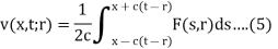
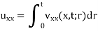
We suppose the function v(x, t;r) which satisfies the equation given below with respect to x and t for t < r,

And the following conditions at t = r
v(x, t;r) = 0, 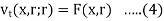
By using D’ Alembert’s solution, the solution of this problem is-
Consider
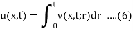
Here we will show that u is the solution,
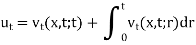
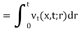
Since 
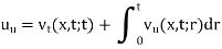
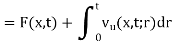
Therefore
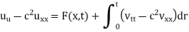

We observe that u(x, t) satisfies the condition (2),
If (2) replaced by

Then the solution of equation (1) is obtained by superposing u from equation (6) on D’Alembert’s solution.

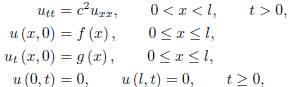
Let us consider the following problem


So f and g are the intital displacement and velocity respectively.
Let us assume the solution of equation (1)
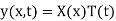
Then

Here the RHS is a function of t while the LHS is function of x, here each of them must be constant and equal to  , therefore


Now from equation (4)
We have

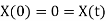
Since T(t) is non-zero, we get X(0) = 0
Similarly y(l, t) = 0 implies that X(l) = 0
Hence we have

Which is an Eigenvalue problem
Case-1:  , the solution of the above eigen value is
Where A and B are the arbitrary constants,
To satisfy the boundary condition
Possibility is A = B = 0,
Hence there is no eigen value  .
.
Case-2:  , the solution of the eigenvalue problem is

The boundary condition implies that A = 0 and A + Bl = 0
Therefore A = B = 0, hence  is not an eigen value.
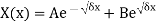
Case-3:  , in this case the solution is

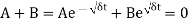
The condition X(0) = 0 implies that A = 0 and X(l) = 0 implies that 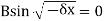
As B = 0 gives the trivial solution, we must have  for a non-trivial solution.
Hence
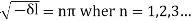

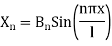
 is called the eigen value and the functions
  are the corresponding eigen functions.
Therefore
For each  , we have
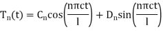
Where  are arbitrary constants, hence
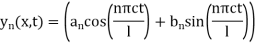
Which is the solution of the equation (1) and satisfies the boundary condition (4)
Vibration of Finite String with Fixed Ends
We know that the solution of the wave equation is

Applying the initial conditions, we have
Solving for  and
and  , we find
Hence
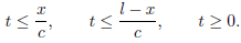
For 0 ≤ x + ct ≤ l and 0 ≤ x − ct ≤ l. The solution is thus uniquely
Determined by the initial data in the region
For larger times, the solution depends on the boundary conditions. Applying
The boundary conditions, we get
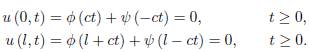
If we set  = −ct, equation first equation of above becomes
 …..(1)
And if we set  = l + ct, the second equation becomes
With  = −
= −
 ……….(2)
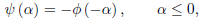
From (1) and (2), we get
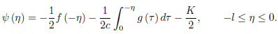
We see that the range of  (
( ) is extended to −l ≤
  ≤ l.
≤ l.
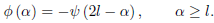
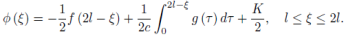
If we put  =
= 
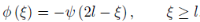
Then, by putting  = 2l −

Heat conduction problem
Let us consider the following heat conduction problem in an infinite rod with the following conditions
- The rod position coincides with the x- axis and the rod is homogenous.
- The heat is uniformly distributed over its cross sections at a time t.
- The surface is isolated to prevent heat loss.
- u(x, t) is the temperature at the point x at time t.
Then the problem we need to solve is


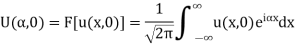
Suppose the Fourier transform of u(x, t) is 
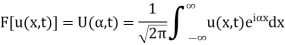
Taking the Fourier transform of equations (1) and assuming that u,  as
as  , we get

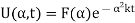
Its solution is given by
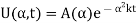
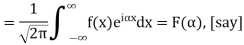
Where  is an arbitrary function to be determined from the initial condition as follows
Hence
By the convolution theorem
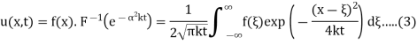
Equations (3) gives the solution of (1) and (2)
Now consider the case k = 1 and
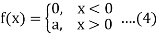
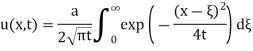
Put
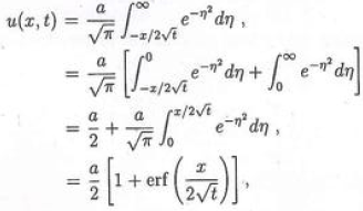
Where erf(x) is the error functions.
References:
1. Erwin Kreyszig, Advanced Engineering Mathematics, 9thEdition, John Wiley & Sons, 2006.
2. Advanced engineering mathematics, by HK Dass
3. Differential equations, Shepley L. Ross, Willey India.
4. Partial differential equations, Phoolan Prasad, Renuka ravindran, John Willey & Sons


