Unit - 1
Rate of convergence
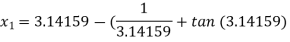
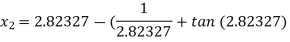
Let  be the given equation. Let α be its exact root.
Then 
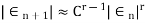
Then the positive number p is said to be order of convergence if,

If p=1, then convergence is linear and if p=2, then it is quadratic.
An iterative method is said to be kth order convergent if k is the largest positive real
Number such that

Here A is a non-zero finite number called asymptotic error constant and it depends on derivative of f(x) at an approximate root x.
 and
and  are the errors in successive approximation.
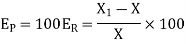
a) Bisection Method: The percentage error  defined by

The rate of convergence for bisection method is 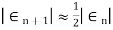
i.e. It converges linearly.
b) Newton Raphson Method: The rate of convergence is


Here p=2, so the convergence is quadratic
c) Secant Method: The rate of convergence is
Order of convergence is non integer and is greater than one , so is super linear.
Note: Order of Convergence
1) Bisection Method : p=1 (linear)
2) Regula-Falsi Method: 1 < p < 2 (super linear).
3) Newton Raphson Method: p = 2 (quadratic).
4) Secant Method: p=1.618 (super linear).
The numerical method provides much wider range to solve the problem that are not possible by analytical methods. There are two ways to solve the numerical methods
a) Exact method: This provides the exact solution of the problem so there will be no error in this.
b) Trial and error or iteration or Approximation method: This will provide the approximate solution that contains certain amount of error which can be tolerated.
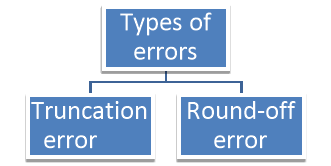
Types of Error:
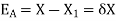
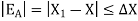
- Absolute Error:
The Approximate error is the numerical difference between the quantity of exact solution and the approximate value of the solution.
Let X be the exact solution and the approximate value of the solution is denoted by  , then the absolute error is defined as
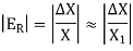
2. Relative Error:
The error obtained by dividing the approximate solution to the exact solution is known as relative error and is denoted by 
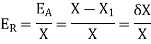
The percentage error is the 100 times of the relative error i.e.
The absolute accuracy is magnitude absolute error.
The relative accuracy is the magnitude of the relative error.
3. Algorithmic Error: A error caused due to rounding off the number or truncation is called algorithmic error.
4. Truncation Error:
The truncation errors are caused by approximated values or on replacing the infinite process to a finite value.
Example: 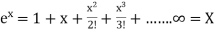 is replaced by
  .
.
Then truncation error is 
5. Round off Error:
The digits that are used to express a number are called significant digits or significant figures.eg  etc.
etc.
In numerical computation, the large number of digits cutting the usual figure is called rounding off. The rule to rounding off is
 in the nth place, leave the nth digit unaltered.
 in the nth place, increase the nth digit =nth digit +1.
 in the nth place, increase the nth digit=nth digit +1 if it is odd; otherwise leave it unchanged.
The number thus rounded-off is said to be correct to n significant figures.
The round off error can be reduced by carrying out the computation to more significant figures at each step of the computation.
Example: Numbers –Round off
 here 0.0003<0.0005 unchanged
 here 0.006>0.005 so, 5=5+1
 here 0.00007>0.00005 so, 8=8+1
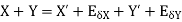
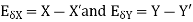
6. Error Propagation:
The error propagation is carried out in the number of steps to get the solution.
The approximate value of the two numbers X and Y is X’ and Y’
Then absolute error is

- Absolute error in addition operation
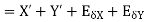
2. Absolute error in subtraction operation
3. Absolute error in multiplication operation
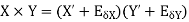
4. Absolute error in division operation
The absolute error  in the quotient of two numbers X and Y
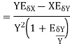
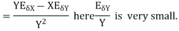
 .
.
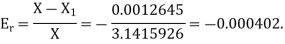
Example: An approximate value of  is given by
 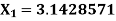 and its exact value is
 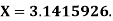 Find the absolute and relative errors.
The absolute error is 
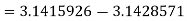
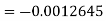 .
.
The relative error is
Example: Find the difference 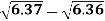 to three significant figure?

Correct to three decimal places.
Example: Round –off the following number to two decimal places

Number | Compare | Changes | Rounded-off number |
48.21416 | 0.004<0.005 | No change | 48.21 |
2.3 742 | 0.004<0.005 | No change | 2.37 |
52.275 | 0.005=0.005 | 0.07+0.01=0.08 | 52.28 |
2.375 | 0.005=0.005 | 0.07+0.01=0.08 | 2.38 |
2.385 | 0.005=0.005 | 0.08+0.01=0.09 | 2.39 |
81.255 | 0.005=0.005 | 0.05+0.01=0.06 | 81.26 |
Example: Find the absolute error if the number  is truncate to three decimal places?
The given number is 
After truncate it to three decimal places the rounded value is 
Therefore the absolute error is 
= 
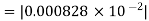
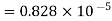 .
.
Generalized error formula (Derivation and Numerical)
Let-
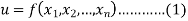
Be the function of  and let the error in each
  be
be  .
.
The error in u is given by-

By using Taylor’s theorem, we expand RHS-
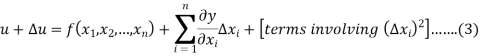
Lets assume that the errors in  are small, so that the higher powers of
  can be neglected,
The above relation yields-
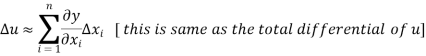
The formula for the relative error follows-

Key takeaways-
- Absolute Error:
The Approximate error is the numerical difference between the quantity of exact solution and the approximate value of the solution.
2. Truncation Error:
The truncation errors are caused by approximated values or on replacing the infinite process to a finite value.
3. Algorithmic Error: A error caused due to rounding off the number or truncation is called algorithmic error.
4. Error Propagation:
The error propagation is carried out in the number of steps to get the solution.
The approximate value of the two numbers X and Y is X’ and Y’
Then absolute error is
The successive approximation is also known as iteration method. To start the solution using this method we need one or more approximate value which is not necessarily the root of the given equation.
We are finding the root of the given equation
 ..(1)
..(1)
We rewrite the given equation in the form
 ..(2)
..(2)
We know that the root of the equation lies between its positive and the negative values
Let 
So, the interval of the root of the equation be  .
.
Now, let  be an approximate root of the given equation (1).
Putting it in equation (2) we get 
Successive substitution give the approximations


…………..

If the above values converge to a definite number then that number will be the root of the given equation.
Example: Find the real root of the equation
Correct to three decimal places in the interval  ]
]
The given equation is  ..(1)
..(1)

Or 
Or 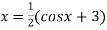 =
=  ..(2)
..(2)
Or 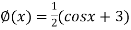
Let  , in the interval
  .
.
The successive approximation we have

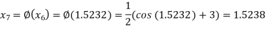
Hence the root of the equation correct to three decimal places is 1.524.
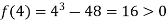
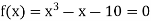
Example: Find the real root of the polynomial 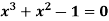 correct to three decimal places?
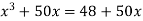
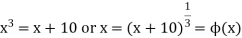
Given equation  ….(1)
….(1)
Here 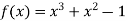
Also 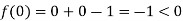
Therefore root of the equation lies between  .
.
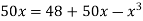
Again 


 ….(2)
….(2)
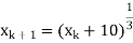
Let  , in the interval
  .
.
The successive approximation we have

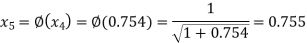
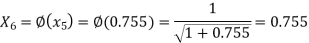
Hence the root of the equation correct to three decimal places is 0.755.
Example: By iteration method, find the value of  , correct to three decimal places.
Let 

Let  .
.
Also 
Therefore the root of the equation lies between 3 and 4.
Given equation can rewrite  .
.

Or 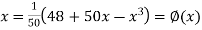 …(2)
…(2)
Let  , in the interval
  .
.
The successive approximation we have


Hence the root of the equation correct to three decimal places is 3.634.
In an initial value problems, we need the solution for  and usually up to a point x = b.
The length of step h for application of any numerical method for the initial value problem should be chosen properly.
There are only two types of errors in computation- truncation and round off error.
We can handle the truncation error but round-off error can be handled, i.e. this is not in the hands of user. They can increase and can destroy the solution too.
Then we say that the method is numerically unstable.
When the step length is chosen larger than the allowed limiting value, in this case we come across with this situation.
Many explicit methods have no restrictions on the step length can be used.
These methods are called unconditionally stable method.
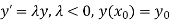
We study the behaviour of the solution of the initial value problem by considering the differential equation in linear form-

The linear form of the problem is given by-
The single step methods are applied in this DE to get the difference equation,
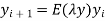
Where  is known as the amplification error.
Note-
When | then all the errors decay and we get a convergent solution.
In this case we say that the method is stable.
Numerical analysis-
Numerical analysis is a branch of mathematics that deal with solving the difficult mathematical problems by using efficient methods
Sometime the mathematical problems are very hard then an approximation to a difficult Mathematical problem is very important to make it more easy to solve numerical approximation has become more popular and a modern tool there are three parts of numerical analysis. The first part of the subject is about the development of a method to a problem. The second part deals with the analysis of the method, which includes the error analysis and the efficiency analysis. Error analysis gives us the understanding of how accurate the result will be if we use the method and the efficiency analysis tells us how fast we can compute the result
The third part of the subject is the development of an efficient algorithm to implement the method as a computer code.
Computers-
“The computer is an electronic device capable of accepting information, applying prescribed processes to the information, and supplying the results of these processes.”
Algorithm-
It is a step-by-step procedure made up of mathematical and/or logical operations designed to solve a particular problem.
Flow-chart-
Flow chart is a pictorial representation of a specific sequence of steps to be used by a computer.
The commonly used symbols in a flow chart-
1.Terminal point
2. Input / Output-
3. Decision logic-

4. Processing operation box-

5. Connector point-

Computer languages-
FORTRAN:
It was introduced by IBM in 1957. FORTRAN stands for FORmula TRANslation.
It is used by most of the scientists and engineers.
It is available on all computers. It has special features like extended double precision, special mathematical functions and complex variables.
C language:
This is a high-level programming language developed by Bell telephone laboratories in 1972.
This programming language is used by large number scientists and engineers.
BASIC:
It was originally developed by John Kemeny and Thomas Kurtz in 1960.
Basically it was used for construction purposes. After sometime it has grown rapidly and the present version is called visual basics.
It is very easy to use.
Mathematical software-
Mathematical software is used to mode, calculate, analyze or visualize the numeric or geometric dataset.
There are various categories of mathematical software for different task relate to mathematical data.
A calculator, which is also a software allows the user to perform simple mathematical calculations such as, addition, subtraction, trigonometry, geometry, exponential, etc. we get the output in text format after entering the data manually.
To solve the algebraic equations, there are various computer algebraic systems. They are especially designed to solve the algebraic equations, and give the accurate solutions.
A lot of computer tools are available to analyze, visualize the statistical data sets, such as R programming, SAS, MS- excel. SPSS, stata, statistica, Julia, dataplot etc.
MATLAB is widely used software for numerical computations. MATLAB stands for MATrics LABoratory. It was developed by Cleve Moler and John N. Little.
It was originally founded to develop a matrix package but today it incorporate various numerical methods such as finding the root of polynomials, Fourier transform, numerical differentiation and integration, ODE, Eigen value and Eigen vectors etc.
It has its own programming language. We can implement the numerical algorithms.
GNU octave is the high-level language, generally made for numerical computations.
We can solve linear and non-linear problems numerically by using it.
- FFTW is a collection of fast C routines for computing the discrete Fourier transform in one or more than one dimensions. It has complex, real and parallel transforms and can handle arbitrary array sizes efficiently.
- LAPACK is a standard library for numerical linear algebra.
- SuperLU is a library which perform an LU decomposition for the direct solution of large and non-symmetric system of linear equations on high performance machines. It is written in C.
There are two types of equations Linear and Non linear equations. Linear equations are those in which dependent variable y is directly proportional to independent variable x and is of degree one. On the other hand non linear equation are those in which y does not directly proportional to x and of degree more than one.
Ex:  +b, where a and b are constant is a linear equation.
 is a non linear equation.
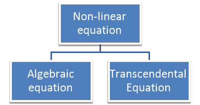
Algebraic Equation:
If f(x) is a pure polynomial, then the equation  is called an algebraic equation in x.
Ex: 
Transcendental Equation:
If f(x) is an expression contain function as trigonometric, exponential and logarithmic etc. Then  is called transcendental equation.
Ex 
Non –linear equation can be solved by using various analytical methods. The transcendental equations and higher order algebraic equations are difficult to solve even sometime are impossible. Finding solution of equation means just to calculate its roots.
Numerical methods are often repetitive in nature. They consist of repetitive calculation of the same process where in each step the result of preceding values are used (substitute). This is known as iteration process and is repeated till the result is obtained to desired accuracy.
The analytical methods used to solve equation; exact value of the root is obtained whereas in numerical method approximate value is obtained.
Bisection method-
This method is consists of finding the root of the equation  which lies between a and b (say).
The function  is continuous function between a and b and f (a) and f (b) are of opposite signs then there is a least one root between a and b.
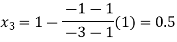
Suppose f (a) is negative and f (b) is positive, then the first approximate value of the root is

If , then the correct root is
  .But if
 , then the root either lies between a and
  or
or  and b according as
  is positive or negative, we again bisect the interval as above and the process is repeated the root is found to desired accuracy.
Example:
Find a real root of 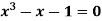 using bisection method correct to five decimal places.
Let  then by hit and trial we have

Thus  .So the root of the given equation should lies between 1 and 2.

Now, 
i.e. positive so the root of the given equation must lies between 

Now, 
i.e. negative so the root of the given equation lies between 

Now, 
i.e. positive so the root of the given equation lies between 

Now, 
i.e. negative so that the root of the given equation lies between 

Now, 
i.e. positive so that the root of the given equation lies between 

Now, 
i.e. positive so that the root of the given equation lies between 

Now, 
I.e. negative so that the root of the given equation lies between 

Now, 
i.e. negative so that the root of the given equation lies between 

Hence the approximate root of the given equation is 1.32421
Example:
Find the root of the equation , using the bisection method.
Let  then by hit and trial we have

Thus  .So the root of the given equation should lies between 2 and 3.

Now, 
i.e. negative so the root of the given equation must lies between 

Now, 
i.e. positive so the root of the given equation must lies between 

Now, 
i.e. negative so the root of the given equation must lies between 

Now, 
i.e. negative so the root of the given equation must lies between 

Now, 
i.e. positive so the root of the given equation must lies between 

Now, 
i.e. negative so the root of the given equation must lies between 

Hence the root of the given equation correct to two decimal place is 2.67965.
Example
Find the root of the equation 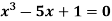 between 2 and 3, using bisection method correct to two decimal place.
Let 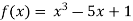
Where 
Thus  .So the root of the given equation should lies between 2 and 3.
Now, 
i.e. positive so the root of the given equation must lies between 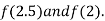
Now, 
i.e. positive so the root of the given equation must lies between 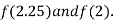
Now, 
i.e. negative so the root of the given equation must lies between 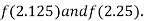
Now, 
i.e. positive so the root of the given equation must lies between 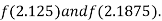
Now, 
i.e. positive so the root of the given equation must lies between 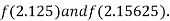
Now, 
i.e. positive so the root of the given equation must lies between 

Now, 
i.e. positive so the root of the given equation must lies between 

Now, 
i.e. positive so the root of the given equation must lies between 

Hence the root of the given equation correct to two decimal place is 2.1269
Regula-Falsi method-
This is the oldest method of finding the approximate numerical value of a real root of an equation .
.
In this method we suppose that  and
and  are two points where
  and
and  are of opposite sign .Let
Hence the root of the equation  lies between
  and
and  and so,
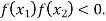
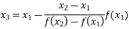
The Regula Falsi formula
Find  is positive or negative. If
  then root lies between
  and
and  or if
or if  then root lies between
  and
and  similarly we calculate
Proceed in this manner until the desired accurate root is found.
Example
Find a real root of the equation 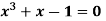 near
near , correct to three decimal place by the Regula Falsi method.
Let 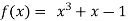
Now, 
And also 
Hence the root of the equation  lies between
  and
and  and so,
By Regula Falsi Method

Now, 
So the root of the equation  lies between 1 and 0.5 and so
By Regula Falsi Method

Now, 
So the root of the equation  lies between 1 and 0.63637 and so
By Regula Falsi Method

Now, 
So the root of the equation  lies between 1 and 0.67112 and so
By Regula Falsi Method

Now, 
So the root of the equation  lies between 1 and 0.63636 and so
By Regula Falsi Method

Now, 
So the root of the equation  lies between 1 and 0.68168 and so
By Regula Falsi Method

Now, 
Hence the approximate root of the given equation near to 1 is 0.68217
Example:
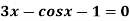
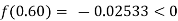
Find the real root of the equation
By the method of false position correct to four decimal places
Let 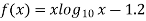
By hit and trail method

 0.23136 > 0
So, the root of the equation  lies between
  2 and
2 and  3 and also
By Regula Falsi Method
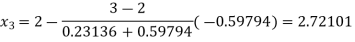
Now, 
So, root of the equation  lies between 2.72101 and 3 and also
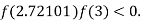
By Regula Falsi Method

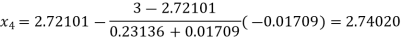
Now, 
So, root of the equation  lies between 2.74020 and 3 and also
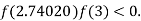
By Regula Falsi Method
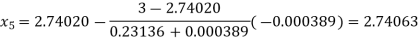
Now, 
So, root of the equation  lies between 2.74063 and 3 and also
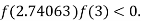
By Regula Falsi Method
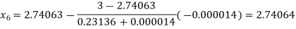
Hence the root of the given equation correct to four decimal places is 2.7406
Example:
Apply Regula Falsi Method to solve the equation
Let 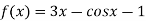
By hit and trail
And 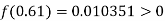
So the root of the equation lies between 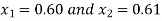 and also
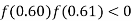
By Regula Falsi Method
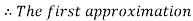
Now, 
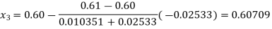
So, root of the equation  lies between 0.60709 and 0.61 and also
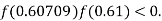
By Regula Falsi Method
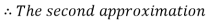

Now, 
So, root of the equation  lies between 0.60710 and 0.61 and also
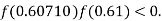
By Regula Falsi Method

Hence the root of the given equation correct to five decimal place is 0.60710.
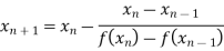
Secant method-
This method is an improvement over the Regula Falsi Method as it does not required the condition 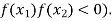
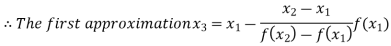
The general formula for successive approximation is,
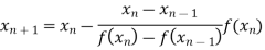
Where 
We keep on calculating until we get desired root to the correct decimal places.
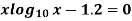
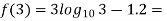
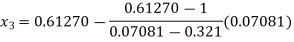
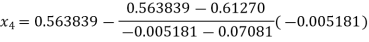
Example: Using the Secant Method find the root of the equation correct to three decimal places

Let 
By Secant Method
Let the initial approximation be 
For n=1, the first approximation 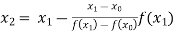
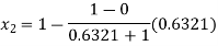

Now, 
For n=2, the second approximation 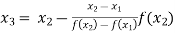
 563839
Now, 
For n=3, the third approximation 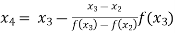
 56717
56717
Now, 
For n=4, the fourth approximation 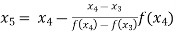
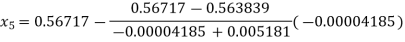
 567143
Hence the root of the given equation correct to four decimal places is 0.5671.
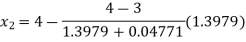
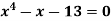
Example: Using the Secant Method to find the root of the equation correct to four decimal places 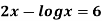
Let 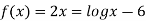
By Secant Method

Let the initial approximation be

For n=1, the first approximation 

Now, 
For n=2, the second approximation 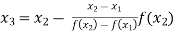
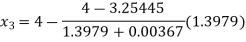

Now, 
For n=3, the third approximation 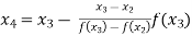
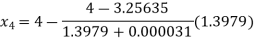

Hence the root of the given equation correct to four decimal places is 3.25636
Example: Using Secant Method find the root of the equation correct to four decimal place
Let 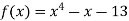
By Secant Method

Let the initial approximation be

For n=1, the first approximation 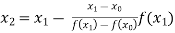
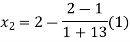

Now, 
So the root of the equation lies between 2 and 1.92857
For n=2, the second approximation ,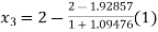

Now, 
So the root of the equation lies between 2 and 1.96590
For n=3, the third approximation

Now, 
So the root of the equation lies between 2 and 1.96600
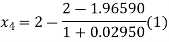
For n=4, the fourth approximation

Now, 
So the root of the equation lies between 2 and 1.96687
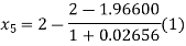
For n=5, the fifth approximation

Now, 
So the root of the equation lies between 2 and 1.96690
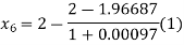
For n=6, the sixth approximation
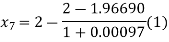

Now, 
Hence the root of the given equation correct to four decimal places is 1.9669.
Let  be the approximate root of the equation
 .
.
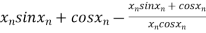
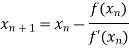
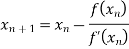
By Newton Raphson formula 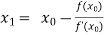
In general,
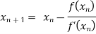
Where n=1, 2, 3…… we keep on calculating until we get desired root to the correct decimal places.
Example: Using Newton-Raphson method, find a root of the following equation correct to 3 decimal places: .
.
Given 

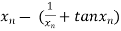
By Newton Raphson Method

= 
=
The initial approximation is 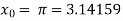 in radian.
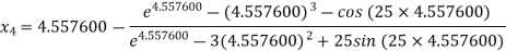
For n =0, the first approximation 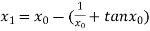

For n =1, the second approximation 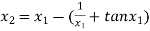

For n =2, the third approximation 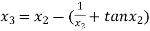
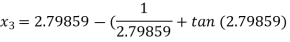

For n =3, the fourth approximation 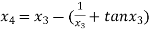
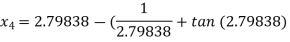
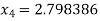
Hence the root of the given equation correct to five decimal place 2.79838.
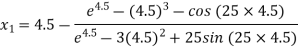
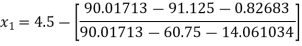
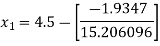
Example: Using Newton-Raphson method, find a root of the following equation correct to 3 decimal places: 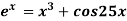 near to 4.5
Let 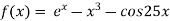

The initial approximation 
By Newton Raphson Method
For n =0, the first approximation 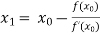

For n =1, the second approximation 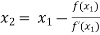
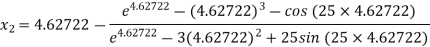
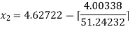
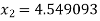
For n =2, the third approximation 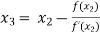
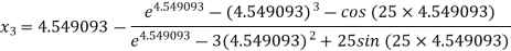
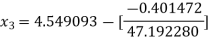
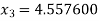
For n =3, the fourth approximation 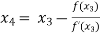

Hence the root of the equation correct to three decimal places is 4.5579
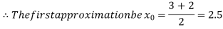
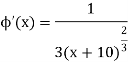
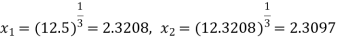
Example: Using Newton-Raphson method, find a root of the following equation correct to 4 decimal places: 
Let 

By Newton Raphson Method
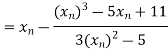
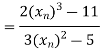
Let the initial approximation be 
For n=0, the first approximation 
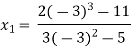
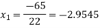
For n=1, the second approximation 
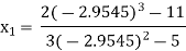

For n=2, the third approximation 
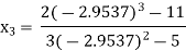

Since  therefore the root of the given equation correct to four decimal places is -2.9537
Fixed point iteration method is also called general iteration method.
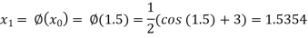
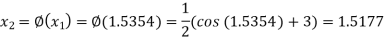
In the very first step in this method, we write the equation f(x) = 0 in an equivalent form such as-

Now we find a root of f(x) = 0 is same as finding a number  such that
  that is a fixed point of
  .
.
Using equation (1), the iteration method can be written as-
The function  is known as the iteration function.
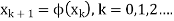
We compute the next approximation as, (starting with the initial approximation)-


...........
...........
...............
................
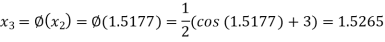
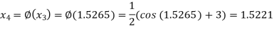
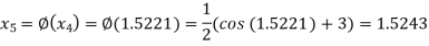
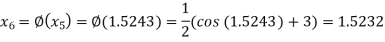
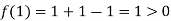
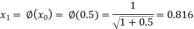
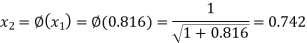
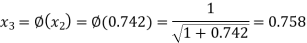
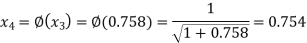
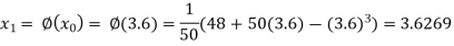
Example: Find the smallest positive root of the equation 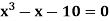 by using fixed point iteration method.
Sol.
Here we have-


Since f(2) f(2) < 0, the smallest positive root lies in the interval (2, 3).
Now write-
We define the iteration method as-
We get-
We find | < 1 for all x in interval (2, 3), hence the iteration converges
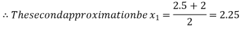
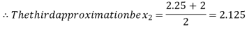
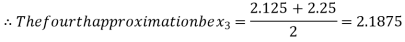
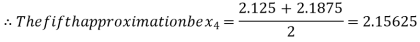
Let
 , we get the following results-

Since

We take the required root as

References:
- E. Kreyszig, “Advanced Engineering Mathematics”, John Wiley & Sons, 2006.
- P. G. Hoel, S. C. Port and C. J. Stone, “Introduction to Probability Theory”, Universal Book Stall, 2003.
- S. Ross, “A First Course in Probability”, Pearson Education India, 2002.
- W. Feller, “An Introduction to Probability Theory and Its Applications”, Vol. 1, Wiley, 1968.
- N.P. Bali and M. Goyal, “A Text Book of Engineering Mathematics”, Laxmi Publications, 2010.
- B.S. Grewal, “Higher Engineering Mathematics”, Khanna Publishers, 2000.


