Unit - 2
Rate of convergence of the above methods
Convergence-
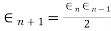
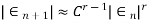
A sequence of iterates  is said to converge with order
 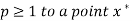 if
if
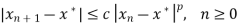
For some constant c > 0.
Note-
- If p = 1, the sequence is said to be linearly convergent to
 .
. - If p = 2, the sequence is said to be quadratically convergent to
 .
. - If p = 3, the sequence is said to be cubically convergent to
 . And so on.
Order and Rate of Convergence
Let  be the given equation. Let α be its exact root.
Then 
Then the positive number p is said to be order of convergence if,

If p=1 , then convergence is linear and if p=2 , then it is quadratic.
a) Bisection Mehtod: The percentage error  defined by
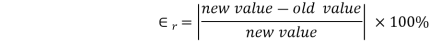
The rate of convergence for bisection method is 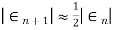
i.e. it converges linearly.
b) Regula-Falsi Method: The rate of convergence is

Here p=1.618 and is linear.
c) Newton Raphson Method: The rate of convergence is


Here p=2 so the convergence is quadratic
d) Secant Method: The rate of convergence is
Order of convergence is non integer and is greater than one , so is super linear.
Note: Order of Convergence
1) Bisection Method : p=1 (linear)
2) Regula-Falsi Method: 1 < p < 2 (superlinear).
3) Newton Raphson Method: p = 2 (quadratic).
4) Secant Method: p=1.618 (superlinear).
Gaussian Elimination Method
In this method we eliminate successively the unknown  so that the equation (1) remain with the single unknown
  and reduce to upper triangular system. At last with help of back substitution we calculate the values of the remaining unknowns.
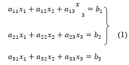
Consider a system of n linear equation in n unknown 


… …… ….. … (1)
… …… …. …

To convert the above system into upper triangular matrix we eliminate  from the second, third, fourth …., n equations above by multiplying the first equation by
 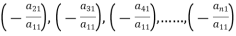 added them to the corresponding equations second, third, fourth,…., n equation. We get

… …… ….. …
… …… …. …
Repeating the above method for  we get finally the upper triangular form.
Upper Triangular form of above


……………………….. (i)

Thus  .
.
Then we calculate the values of  .
.
Note: In (i) the coefficient  is the pivot element and the equation is called the pivot equation. If
  then the above method fails and if it is close to zero the round off error may occur.
If  or very small compared to other coefficient of the equation, then we find the largest available coefficient in the column given below the pivot equation and then interchange the two rows to obtain new pivot variable this is known as partial pivoting.
Example1 Apply Gauss Elimination method to solve the equations:

Given Check Sum (sum of coefficient and constant)
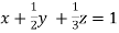
 -1 …. (I)
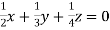
 -16 …. (ii)
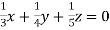
 5 …. (iii)
(I)We eliminate x from (ii) and (iii)
Apply eq(ii)-eq(i) and eq(iii)-3eq(i) we get
 -1 ….(i)
 -15 ….(iv)
 8 ….(v)
(II) We eliminate y from eq(v)
Apply 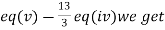
 -1 ….(i)
 -15 ….(iv)
 73 ….(vi)
(III) Back Substitution we get
From (vi) we get 
From (iv) we get 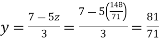
From (i) we get 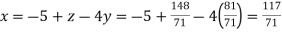
Hence the solution of the given equation is 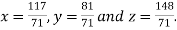
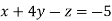
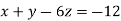
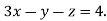
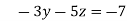
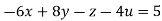
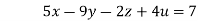
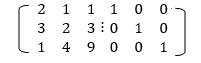
Example2 Solve the equation by Gauss Elimination Method:

Given 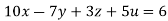

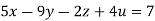
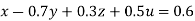
Rewrite the given equation as
 … (i)
… (i)
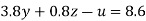
 ….(ii)
 ….(iii)
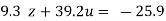
 …(iv)
…(iv)
(I) We eliminate x from (ii),(iii) and (iv) we get
Apply eq(ii) + 6eq(i), eq(iii) -3eq(i), eq(iv)-5eq(i) we get
 …(i)
…(i)
 ….(v)
….(v)
 ….(vi)
 …(vii)
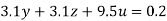
(II) We eliminate y from (vi) and (vii) we get
Apply 3.8 eq(vi)-3.1eq(v) and 3.8eq(vii)+5.5eq(v) we get
 …(i)
…(i)
 ….(v)
….(v)
 …(viii)
 …(ix)
…(ix)
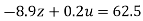
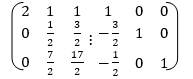
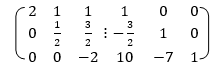
(III) We eliminate z from eq (ix) we get
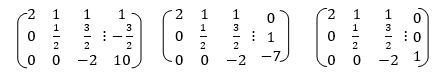
Apply 9.3eq (ix) + 8.3eq (viii), we get
 … (i)
… (i)
 ….(v)
….(v)
 …(viii)
350.74u=350.74
Or u = 1
(IV) Back Substitution
From eq(viii) 
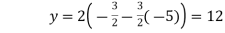
Form eq(v), we get 
From eq(i), 
Hence the solution of the given equation is x=5, y=4, z=-7 and u=1.
Example3 Apply Gauss Elimination Method to solve the following system of equation:

Given  … (i)
… (i)
 … (ii)
 … (iii)
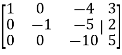
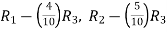
(I) We eliminate x from (ii) and (iii)
Apply 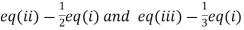 we get
 … (i)
… (i)
 … (iv)
 … (v)
… (v)
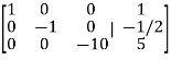
(II) We eliminate y from (v)
Apply we get
 … (i)
… (i)
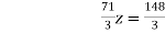
 … (vi)
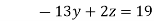
 … (vii)
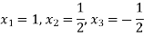
(III) Back substitution
From (vii) 
From (vi) 
From (i) 
Hence the solution of the equation is 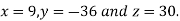
Example4: Solve the system by Gauss Elimination method using partial pivoting

Given exact solution is 
Given equations are 

Using partial pivoting we rewrite the given equations as
 (1)
(1)
 (2)
(2)
Using Gauss elimination method
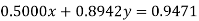
Multiplying (1) by (-0.0003120/0.5000) + (2) we get
Or 
Substituting value of y in equation (1) we get 
Hence 
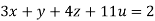
Example5: Solve the system of linear equations


Using partial pivoting by Gauss elimination method we rewrite the given equations as
 (1)
(1)
 (2)
(2)
 (3)
(3)
Apply  and
and 
 (1)
(1)
 (4)
(4)
 (5)
(5)
Apply  )
)
 (1)
(1)
 (4)
(4)
Or  .
.
Putting value of z in  we get
  .
.
Putting values of y and z in  we get
  .
.
Hence the solution of the equation is  .
.
Gauss-Jordan method-
In this method we reduce the given system of equations AX = b to a diagonal system of equations Ix = d, here I is the identity matrix.
The reduced system gives the solution vector X.
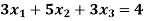
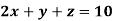
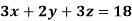
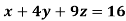
Example: By using Gauss-Jordan method, solve the system of equations-
Sol:
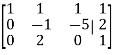
Here the augmented matrix will be-

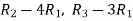
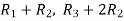
By performing elementary row transformation, and eliminations, we get-
Now making the pivots as 1, ((
We obtain,

Hence the solution of the system is-
Matrix Inversion using Gauss Jordan method-
We know that X will be the inverse of a matrix A if

Where I is an identity matrix of order same as A.
We write , using elementary operation we covert the matrix A in to a upper triangular matrix. Then compare this matrix with each corresponding column and using back substitution.
The determinant of this coefficient matrix is the product of the diagonal elements of the upper triangular matrix.
If this |A|=0 then inverse does not exist.
Example1
Solve the system of equations
Here A =
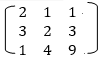
The augmented system is
Apply 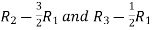
Apply 
Here 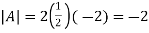
Which is non zero so the inverse exists.
Comparing the diagonal matrix with corresponding columns.
By back Substitution we get
Form first part of above 
Similarly we solve second and third part and obtain a matrix whose columns are
Which is the required inverse 
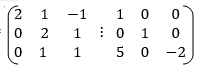
Example2: Find the inverse and determinant of-

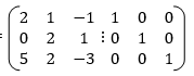
Let [A:I]= 
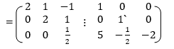
Apply 
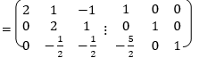
Apply 
= 
Apply 
Here 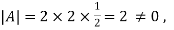 therefore
  exist.
On comparing the coefficient matrix with each column of RHS matrix.
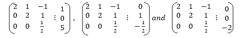
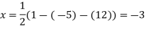
From first term back substitution


We get 
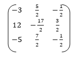
From second and third we get 
Hence 
Jacobi’s Iteration method:
Let us consider the system of simultaneous linear equation
The coefficients of the diagonal elements are larger than the all other coefficients and are non zero. Rewrite the above equation we get
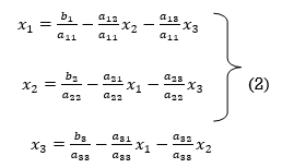
Take the initial approximation 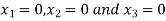 we get the values of the first approximation of
 .
.
By the successive iteration we will get the desired the result.
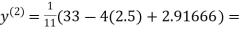
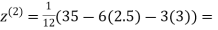
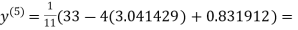
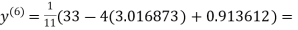
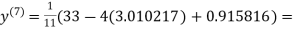
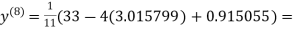
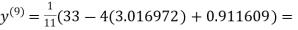
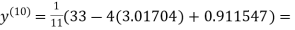
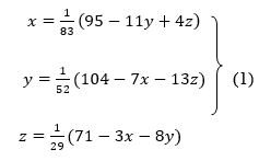
Example: Use Jacobi’s method to solve the system of equations:

Since 
So, we express the unknown with large coefficient in terms of other coefficients.
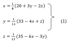
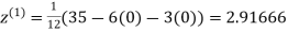
Let the initial approximation be 

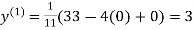


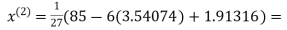
 2.35606
 0.91666


 1.932936
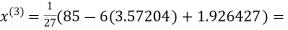
 0.831912

 3.016873
 1.969654


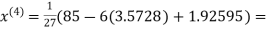
 3.010217
 1.986010


 1.988631
 0.915055


 1.986532
 0.911609


 1.985792
 0.911547


 1.98576
 0.911698
Since the approximation in ninth and tenth iteration is same up to three decimal places, hence the solution of the given equations is 
Example: Solve by Jacobi’s Method, the equations

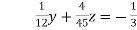
Given equation can be rewrite in the form
 … (i)
… (i)
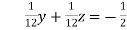
 ..(ii)
 ..(iii)
Let the initial approximation be 

Putting these values on the right of the equation (i), (ii) and (iii) and so we get


Putting these values on the right of the equation (i), (ii) and (iii) and so we get


Putting these values on the right of the equation (i), (ii) and (iii) and so we get
 0.90025


Putting these values on the right of the equation (i), (ii) and (iii) and so we get


Putting these values on the right of the equation (i), (ii) and (iii) and so we get


Hence solution approximately is 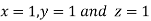
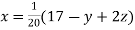
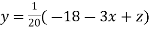
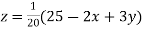
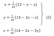
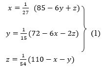
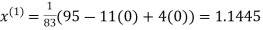
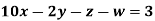
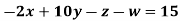
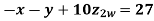
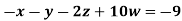
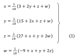
Example: Use Jacobi’s method to solve the system of the equations

Rewrite the given equations
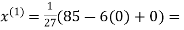
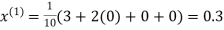
Let the initial approximation be 

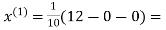 1.2
1.2
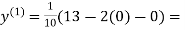 1.3
1.3
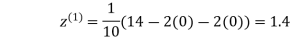

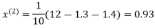
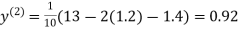
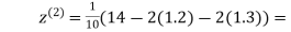 0.9
0.9

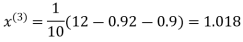
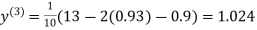
 1.03
1.03

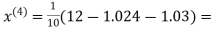 0.9946
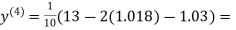 0.9934
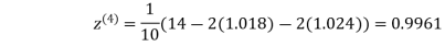

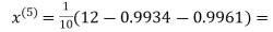 1.0015

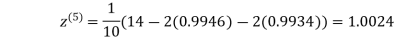
Hence the solution of the above equation correct to two decimal places is
Gauss Seidel method:
This is the modification of the Jacobi’s Iteration. As above in Jacobi’s Iteration, we take first approximation as  and put in the right hand side of the first equation of (2) and let the result be
  . Now we put
  right hand side of second equation of (2) and suppose the result is
  now put
  in the RHS of third equation of (2) and suppose the result be
  the above method is repeated till the values of all the unknown are found up to desired accuracy.
Example: Use Gauss –Seidel Iteration method to solve the system of equations

Since 
So, we express the unknown of larger coefficient in terms of the unknowns with smaller coefficients.
Rewrite the above system of equations
Let the initial approximation be 

 3.14814


 2.43217


 2.42571


 2.4260


Hence the solution correct to three decimal places is

Example: Solve the following system of equations
 By Gauss-Seidel method.
Rewrite the given system of equations as
Let the initial approximation be 


Thus the required solution is 
Example: Solve the following equations by Gauss-Seidel Method
Rewrite the above system of equations
Let the initial approximation be 


Hence the required solution is 
Solving Eigen value problems (Power method)-
Consider the eigen value problem

The Eigen values of a matrix A are given by the roots of the characteristic equation
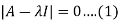
If the matrix A is of order n, then expanding the determinant, we obtain the characteristic equation as

For the given matrix we write the characteristic equation, by expanding we find the roots  . These are called the Eigen values.
Now suppose  be the solution of the system of homogeneous equations, corresponding to the Eigen value
These vectors  are called the Eigen vectors.
To find the approximate values of all the Eigen values and Eigen vectors, iteration method or power method is used.
Power method is used when only the largest and/or the smallest Eigen values of a matrix are desired.
Procedure for Power method-
Step-1: First we choose an arbitrary real vector  , basically
  is chosen as-

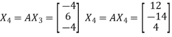
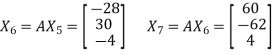
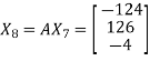
Step-2: Compute  ,
,  ,
,  ,
,  , …………
 Put
Put 
Step-3: Compute  ,
,  ,
, 
Step-4: The largest Eigen value is

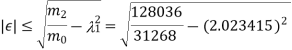
The error in  can be find as-
The Eigen vector corresponding to  is
is 
How do we determine the smallest Eigen value?
If  is the Eigen value of A, then the reciprocal
  is the Eigen value of
  , then the reciprocal of the largest Eigen value of
  will be the smallest Eigen value of A.
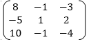
Example: Find the largest Eigen value and the corresponding Eigen vector of the matrix
Also find the error in the value of the largest Eigen value.
Sol.
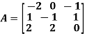
Let us choose the initial vector

Then
 and
and 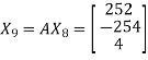
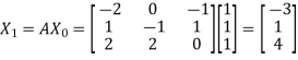
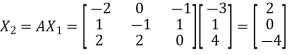
Now put  , then-
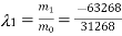
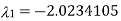
Hence the largest Eigen value is-
And the corresponding Eigen vector is-

The error can be calculated as-

References:
- E. Kreyszig, “Advanced Engineering Mathematics”, John Wiley & Sons, 2006.
- P. G. Hoel, S. C. Port and C. J. Stone, “Introduction to Probability Theory”, Universal Book Stall, 2003.
- S. Ross, “A First Course in Probability”, Pearson Education India, 2002.
- W. Feller, “An Introduction to Probability Theory and Its Applications”, Vol. 1, Wiley, 1968.
- N.P. Bali and M. Goyal, “A Text Book of Engineering Mathematics”, Laxmi Publications, 2010.
- B.S. Grewal, “Higher Engineering Mathematics”, Khanna Publishers, 2000.


