Unit - 3

Polynomial interpolation

3.1 Polynomial interpolation: Existence uniqueness of interpolating polynomials

Interpolation

Definition:

Interpolation  is a technique of  estimating the value of  a  function for any  intermediate value of the  independent  variable while  the process  of  computing the  value of the function outside the given range is called   extrapolation.

Let be a function of x.

The table given below gives corresponding values of y for  different values of x.

X				….
y= f(x)				….

The process of finding the values of y corresponding to any value of x which lies between   is called interpolation.

If the given function is a polynomial it is polynomial interpolation and given function is known as interpolating polynomial.

Note- The process of computing the value of the function outside the given range is called extrapolation.

Thus interpolation is the “art of reading between the lines of a table.”

Conditions for Interpolation

1)     The function must be   a polynomial of independent variable.

2)     The function   should be either increasing or decreasing function.

3)     The value of   the function should be increase or decrease uniformly.

Finite Difference

Let be a function of x.The table given below gives corresponding values of y for  different values of x.

X				….
y= f(x)				….

There are three types of differences are useful-

a)     Forward Difference: 

The  are called differences of y, denoted by 

The  symbol   is  called the forward  difference operator.  Consider the forward  difference  table  below:

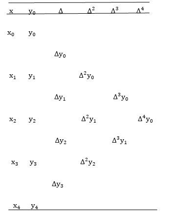
Where

And third forward difference  so  on.

b)    Backward Difference:

The difference are called first backward difference and  is denoted by  Consider the backward  difference  table  below:

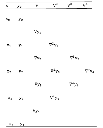
Where

And 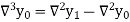third backward differences so on.

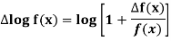
Example: Construct a backward difference table for y = log x, given-

Sol. The backward difference table will be-

10   20   30   40   50	1   1.3010   1.4771   1.6021   1.6990	0.3010   0.1761   0.1250   0.0969	-0.1249   -0.0511   -0.0281	0.0738   0.0230	-0.0508

3.2 Lagrange and Newton’s divided difference interpolation

Divided Difference:

In the case of interpolation, when the value of the arguments are not equi-spaced (unequal intervals) we use the class of differences called divided differences.

Definition:   The   difference which are defined by taking into consideration   the change in the value of the argument are known as divided differences.

Let be a function defined as

			…….
			…………

Where are unequal i.e. it is case of unequal interval.

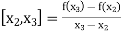
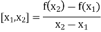
The first order divided differences are:

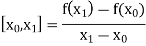
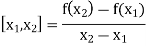
And so on.

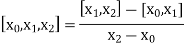
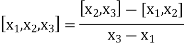
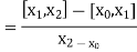
The second order divided difference is:

And so on.

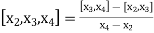
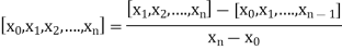
Similarly the nth order divided difference is:

With the help of these we construct the divided difference table:

X	f(x)

Newton’s Divided difference Formula:

Let be a function defined as

			…….
			…………

Where are unequal i.e. it is case of unequal interval.

.

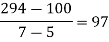
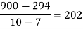
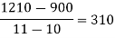
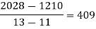
Example1: By means of Newton’s divided difference formula, find the values of from the following table:

We construct the divided difference table is given by:

x	f(x)	First order divide difference	Second order divide difference	Third order divide difference	Fourth order divide difference
4   5   7   10   11   13	48   100   294   900   1210   2028				0      0

By Newton’s Divided difference formula

.

Now, putting in above we get

.

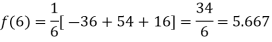
Example2: The following values of the function f(x) for values of x are given:

Find the value of and also the value of x for which f(x) is maximum or minimum.

We construct the divide difference table:

x	f(x)	First order divide difference	Second order divide difference	Third order divide difference
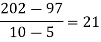
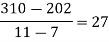
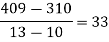
1   2   7   8	4   5   5   4			0

By Newton’s divided difference formula

.

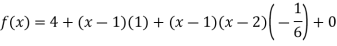
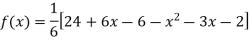
Putting  in above we get

For maximum and minimum of , we have

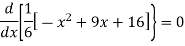
Or 

Example3: Find a polynomial satisfied by

, by the use of Newton’s interpolation formula with divided difference.

Here

We will construct the divided difference  table:

x	F(x)	First order divided difference	Second order divided difference	Third order divided difference	Fourth order divided difference
-4   -1   0   2   4	1245   33   5   9   1335

By Newton’s divided difference formula

.

This is the required polynomial.

Lagrange’s Interpolation of polynomial:

Let , be defined  function we get

X				…..
f(x)				……

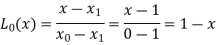
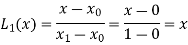
Where the interval is not necessarily equal. We assume f(x) is a polynomial od degree n.  Then Lagrange’s interpolation formula is given by

Example1: Deduce Lagrange’s formula for interpolation.  The observed values of a function  are respectively  168,120,72 and 63 at the  four position3,7,9 and 10 of  the independent variable. What  is the  best estimate you can for  the value of the  function  at the position6 of  the independent variable.

We construct  the table for the given data:

We need to  calculate for  x =  6, we need f(6)=?

Here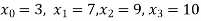

We get

By Lagrange’s interpolation formula,  we have

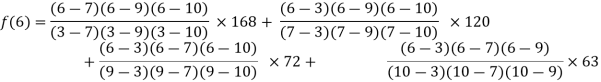
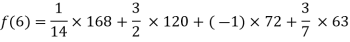
Hence the estimated value for x=6 is 147.

Example2: By means of Lagrange’s formula, prove that

We construct the table:

X	0	1	2	3	4	5	6
Y=f(x)

Here x = 3, f(x)=?

By Lagrange’s formula for   interpolation

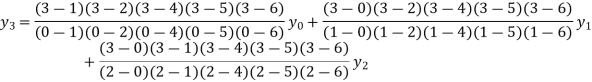
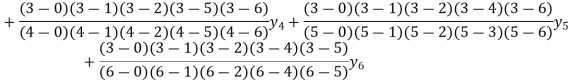
Hence proved.

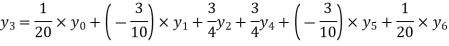
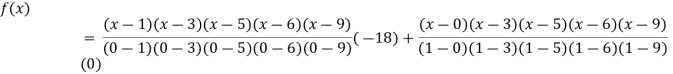
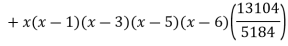
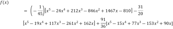
Example3: Find the polynomial  of  fifth degree from  the following data

Here

We get 

By Lagrange’s  interpolation  formula

Key takeaways-

1. The   difference which are defined by taking into consideration   the change in the value of the argument are known as divided differences.
2. Newton’s Divided difference Formula

.

3.3 Error in interpolation, Central difference & averaging operators

Error in interpolation:

We know that, the interpolation means to estimate a missing function value by taking a weighted average of known function value at neighbouring points.

Let y = f(x) is the known function at (n + 1) points.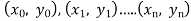

A polynomial of degree n. is known as the interpolating polynomial when passes through these (n + 1) points.

can be constructed using only the numerical values and and does not need any order derivatives of f (x). The approximation is known as interpolated value when and extrapolated value when or .

Note- Error increases when the number of interpolation is increased.

The error of the polynomial is obtained by the generalized Rolle’s theorem,

It is given as-

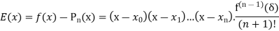
Here contains {x, }

Note- that the error term given above is same for Lagrange polynomial and interpolating polynomial obtained from divide difference table

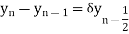
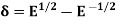
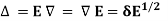
Central differences:

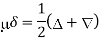
The central difference operator is defined by the relations,

...................

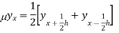
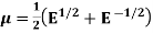
Averaging operator (:

It is defined as-

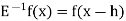
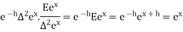
Shift operator E:

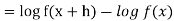
It is the operation of increasing the argument x by h so that

Ef(x) = f(x + h)

f(x) = f(x + 2h) and so on.

The inverse operator is defined by

Note:
1.

2.

3.

4.

5.

6.

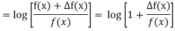
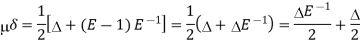
Example: Prove that

Sol.

By taking left hand side, we get-

Example: Prove that-

Sol.

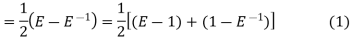
From (1)-

Hence proved.

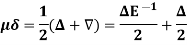
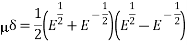
Example: Prove that

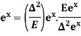
Sol.

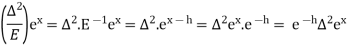
R.H.S

3.4 Gauss-forward and backward difference interpolation

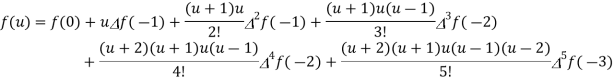
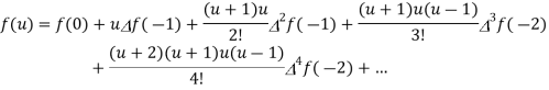
Gauss forward difference formula-

1. Gauss forward difference formula-

2.     Gauss backward difference formula-

Example: By using Gauss forward difference formula obtain f(32) given that-

f(25) = 0.2707   f(35) = 0.3386

f(30) = 0.3027   f(40) = 0.3794

Sol.

Here

Let us take the origin at 30, a = 30 then we get-

u = 0.4

The forward difference table-

u	x	F(x)
-1   0   1   2	25   30   35   40	0.2707   0.3027   0.3386   0.3794	0.032   0.359   0.408	0.0039   0.0049	0.0010

By using Gauss forward difference formula, we get-

Example: Find by using Gauss forward formula if-

Sol.

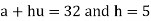
Let a = 8, h = 4,

We have

a + hu = 9

And we get-

u = 0.25

The forward difference table-

u	X	F(x)
-2   -1   0   1   2	0   4   8   12   16	14   24   32   35   40	10   8   3   5	-2   -5   2	-3   7	10

By using Gauss forward difference formula, we get-

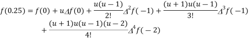
Hence

Example: Using Gauss’s backward interpolation formula, find the population for the year 1936 given that-

Sol.

Let origin is at 1941 and h = 10

Then-

Which gives-

The backward difference table-

u	F(u)
-4   -3   -2   -1   0   1	12   15   20   27   39   52	3   5   7   12   13	2   2   5   1	0   3   -4	3   -7	-10

By using Gauss backward formula, we get-

thousands

Hence the pop. Of the year 1936 is 32625

Key takeaways-

1. Gauss forward difference formula-

2. Gauss backward difference formula-

3.5 Hermite and Spline interpolation, piecewise polynomial interpolation

Hermite’s interpolation formula-

The Hermite’s interpolation formula is defined as-

Example: Find the cubic polynomial by using Hermite’s interpolation formula, given-

0	0	0
1	1	1

Sol.

We know that Hermite’s interpolation formula-

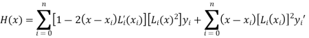
..........(1)

Now

And

Hence

From equation (1)-

and

Spline interpolation-

The approximation of arbitrary functions on a closed interval becomes oscillatory for higher-degree polynomials. By dividing the given interval into a collection of subintervals, piecewise polynomial approximation consists of constructing a different approximating polynomial on each subinterval. Cubic spline interplation is the most common piecewise approximation using cubic polynomial, known as spline function, connecting each pair of data points. Cubic splines are third-order curves employed to connect each pair of data points.

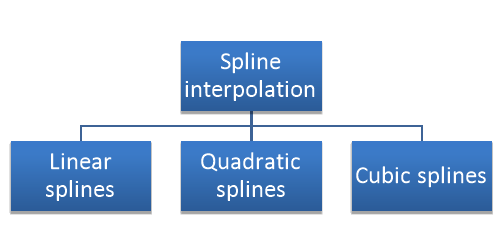
Linear splines-

This type of spline defined by a function that is the linear function.

Linear splines are called first order splines.

Consider a set of (n + 1) data points, (

The set of linear functions defining linear splines in n intervals are-

………………………………………….

………………………………………….

………………………………………….

………………………………………….

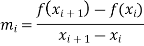
is the slope if the line connects the data points .

is given as-

Quadratic splines:

These are called the second order splines.

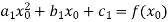
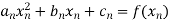
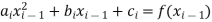
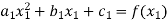
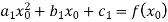
For each interval, we fit a parabola give by-

For n + 1 data points we have n intervals. So we should determine 3 × n unknown constants. The 3n condition to find the 3n unknowns are given by the following equations.

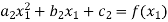
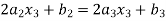
1. At the interior knots, the function values must be-

For i = 2, n giving raise to 2(n − 1) = 2n – 2 conditions.

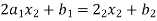
2.     The first and last functions must pass through the two end points

Giving two conditions.

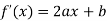
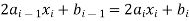
3.     At the interior knots, the first derivatives f (x) = 2ax + b must be equal.

For i = 2 to n giving n − 1 conditions

4.     Assume that the second derivative is zero at the first point. Then the first two points are connected by a straight line, so

Thus solving (2n − 2) + 2 + (n − 1) + 1 = 3n conditions above we obtain the 3n unknown constants a, b and c.

Cubic splines-

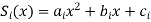
Let us fit a third order polynomial,

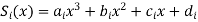
For each of the n intervals between the (n + 1) data points (knots) (i = 0, 1, 2, . . . n). The problem is to find the 4 × n = 4n unknown constants

We have the following conditions-

1. 2n − 2 conditions since the function values must be equal at the (n − 1) interior knots.
2. 2 conditions since the first and last functions must pass through the two end points x0 and xn.
3. (n − 1) conditions since the first derivatives must be equal at the (n − 1) interior points.
4. (n − 1) conditions since the second derivatives must be equal at the (n − 1) interior knots.

The above conditions are summed to (2n − 2) + (2) + (n − 1) + (n − 1) = 4n − 2, thus short of 2 more conditions to solve the 4n unknown constants.

Natural spline for which the end point constraints are assumed as “second derivatives at the end knots are zero”.

Natural splines are more frequently used in which the end cubic approach linearity at their extremities.

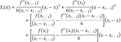
The cubic spline for each interval (, ) is given by

There are only two unknowns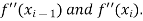

Therefore the second derivatives at the end points of the interval can be find by the following equations,

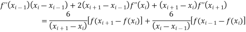
This equation written for the (n -1) interior points results in (n −1) simultaneous equations for the second derivatives.

Example: Fit a linear spline of the data given below:

Sol.

Here we have, n = 4 and there are 3 intervals.

Let us assume that-

,     ,       ,       

,     ,       ,       

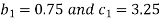
And the slope,

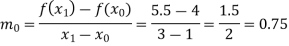
Similarly we can find,

As we know that the

The three splines will be-

Example: Fit quadratic splines for the following data.

Sol.

For the 4 data points in 3 intervals, we fix three splines of the form-

We need to find 9 unknown (3 * 3 = 9).

We need 9 conditions to determine 9 unknowns.

There are 2 interior points .

1. Function value must be equal at the two interior points, giving rise to four equations.

For i=2 to 3

For i=2

For

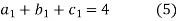
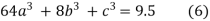
2.     The first and last function must pass through the end points and giving rise to two equations-

Or

3.     The third derivative at the interior knots must be equal-

For i=2,3

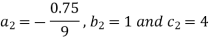
4.     Assume that the second derivative is zero at the first point i.e.,

Using (9), in (1) and(5)-

We get-

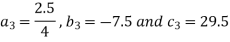
By solving second and third equation, we get-

By solving 4 and 6, we get-

So that we get the values of 9 coefficients-

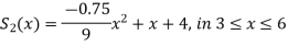
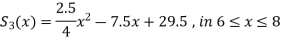
Now-

The three quadratic splines will be-

References:

1. E. Kreyszig, “Advanced Engineering Mathematics”, John Wiley & Sons, 2006.
2. P. G. Hoel, S. C. Port and C. J. Stone, “Introduction to Probability Theory”, Universal Book Stall, 2003.
3. S. Ross, “A First Course in Probability”, Pearson Education India, 2002.
4. W. Feller, “An Introduction to Probability Theory and Its Applications”, Vol. 1, Wiley, 1968.
5. N.P. Bali and M. Goyal, “A Text Book of Engineering Mathematics”, Laxmi Publications, 2010.
6. B.S. Grewal, “Higher Engineering Mathematics”, Khanna Publishers, 2000.