Unit - 4
Numerical Integration
Numerical Integration
Numerical integration is a process of evaluating or obtaining a definite integral  from a set of numerical values of the integrand f(x).In case of function of single variable, the process is called quadrature.
Newton cotes formula-
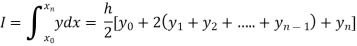
Suppose  where y takes the values
And let the integration interval (a,b) is divided into n equal sub-intervals, each of width h = b – a /n, so that,


The above formula is known as Newton’s cotes formula.
This is also known as general Quadrature formula.
Trapezoidal Method:
Let the interval [a,b] be divided into n equal intervals such that  <
< <….<
<….< =b.
=b.
Here  .
.
To find the value of  .
.
Setting n=1, we get
Or I = 
The above is known as Trapezoidal method.
Note: In this method second and higher difference are neglected and so f(x) is a polynomial of degree 1.
Geometrical Significance: The curve y=f(x),is replaced by n straight lines with the points  (
( );(
);( ) and (
 );…….;(
 ) and (
 ).
).
The area bounded by the curve y=f(x), the ordinates  ,and the x axis is approximately equivalent to the sum of the area of the n trapeziums obtained.
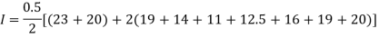
Example1: State the trapezoidal rule for finding an approximate area under the given curve. A curve is given by the points (x, y) given below:
(0, 23), (0.5, 19), (1.0, 14), (1.5, 11), (2.0, 12.5), (2.5, 16), (3.0, 19), (3.5, 20), (4.0, 20).
Estimate the area bounded by the curve, the x axis and the extreme ordinates.
We construct the data table:
X | 0 | 0.5 | 1.0 | 1.5 | 2.0 | 2.5 | 3.0 | 3.5 | 4.0 |
Y | 23 | 19 | 14 | 11 | 12.5 | 16 | 19 | 20 | 20 |
Here length of interval h =0.5, initial value a = 0 and final value b = 4
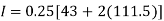
By Trapezoidal method
Area of curve bounded on x axis =

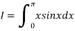
Example2: Compute the value of 
Using the trapezoidal rule with h=0.5, 0.25 and 0.125.
Here 
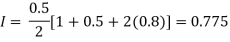
For h=0.5, we construct the data table:
X | 0 | 0.5 | 1 |
Y | 1 | 0.8 | 0.5 |
By Trapezoidal rule

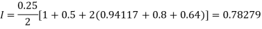
For h=0.25, we construct the data table:
X | 0 | 0.25 | 0.5 | 0.75 | 1 |
Y | 1 | 0.94117 | 0.8 | 0.64 | 0.5 |
By Trapezoidal rule

For h = 0.125, we construct the data table:
X | 0 | 0.125 | 0.25 | 0.375 | 0.5 | 0.625 | 0.75 | 0.875 | 1 |
Y | 1 | 0.98461 | 0.94117 | 0.87671 | 0.8 | 0.71910 | 0.64 | 0.56637 | 0.5 |
By Trapezoidal rule

 [(1+0.5)+2(0.98461+0.94117+0.87671+0.8+0.71910+0.64+0.56637)]

Example3: Evaluate using trapezoidal rule with five ordinates
Here 
We construct the data table:
X | 0 |  |  |  |  |  |
Y | 0 | 0.3693161 | 1.195328 | 1.7926992 | 1.477265 | 0 |


Simpson’s Rule:
Let the interval [a,b] be divided into n equal intervals such that  <
< <….<
<….< =b.
=b.
Here  .
.
To find the value of  .
.
Setting n = 2,

Which is known as Simpson’s 1/3- rule or Simpson’s rule.
Note: In this rule third and higher differences are neglected so f(x) is a polynomial of degree 2.
Example1: Estimate the value of the integral

By Simpson’s rule with 4 strips and 8 strips respectively.
For n=4, we have 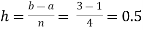
E construct the data table:
X | 1.0 | 1.5 | 2.0 | 2.5 | 3.0 |
Y=1/x | 1 | 0.66666 | 0.5 | 0.4 | 0.33333 |
By Simpson’s Rule


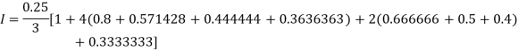
For n = 8, we have 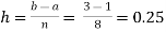
X | 1 | 1.25 | 1.50 | 1.75 | 2.0 | 2.25 | 2.50 | 2.75 | 3.0 |
Y=1/x | 1 | 0.8 | 0.66666 | 0.571428 | 0.5 | 0.444444 | 0.4 | 0.3636363 | 0.333333 |
By Simpson’s Rule


Example2: Evaluate 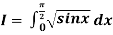 Using Simpson’s 1/3 rule with
  .
.
For  , we construct the data table:
X | 0 |  |  |  |  |  |  |
 | 0 | 0.50874 | 0.707106 | 0.840896 | 0.930604 | 0.98281 | 1 |
By Simpson’s Rule


Example3: Using Simpson’s 1/3 rule with h = 1, evaluate

For h = 1, we construct the data table:
X | 3 | 4 | 5 | 6 | 7 |
 | 9.88751 | 22.108709 | 40.23594 | 64.503340 | 95.34959 |
By Simpson’s Rule


= 177.3853
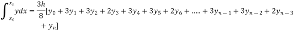
Simpson’s 3/8 rule
Let the interval [a,b] be divided into n equal intervals such that  <
< <….<
<….< =b.
=b.
Here  .
.
To find the value of  .
.
Setting n=3, we get
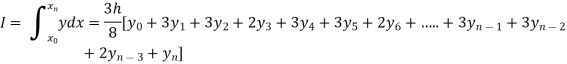
Is known as Simpson’s 3/8 rule which is not as accurate as Simpson’s rule.
Note: In this rule the fourth and higher differences are neglected and so f(x) is a polynomial of degree 3.
Example1: Evaluate 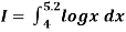
By Simpson’s 3/8 rule.
Let us divide the range of the interval [4, 5.2] into six equal parts.
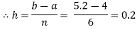
For h=0.2, we construct the data table:
X | 4.0 | 4.2 | 4. 4 | 4.6 | 4.8 | 5.0 | 5.2 |
Y=logx | 1.3863 | 1.4351 | 1.4816 | 1.5261 | 1.5686 | 1.6094 | 1.6487 |
By Simpson’s 3/8 rule
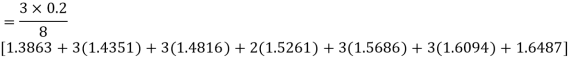
= 1.8278475
Example2: Evaluate 
Let us divide the range of the interval [0,6] into six equal parts.
For h=1, we construct the data table:
X | 0 | 1 | 2 | 3 | 4 | 5 | 6 |
 | 1 | 0.5 | 0.2 | 0.1 | 0.0588 | 0.0385 | 0.027 |
By Simpson’s 3/8 rule

 +3(0.0385)+0.027]
=1.3571
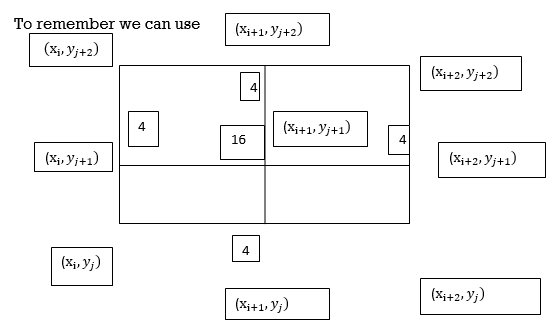
Double Integration: Trapezoidal Method
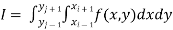
The double integration is defined by

Where .
.
Trapezoidal Rule:
The double integration is defined by
Where .
.

Or

Also the double integration is defined by
Where .
.

Again Applying Trapezoidal rule to each term with respect to y.
Example1: Evaluate 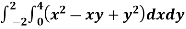
Let 
Here the interval of x and y are  and
and  .
.
Let 
Consider the following table:
 |
 |
 |
 |
 |

|
 |
 |
 |
 |
 |
 |
 |
 |
 |
 |
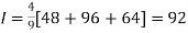
By Trapezoidal Rule


 .
.
Example2: Evaluate 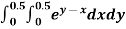
Let 
Here 
Let the number of interval be  .
.

 |
 |
 |
 |
 |

|
 |
 |
 |
 |
 |
 |
 |
 |
 |
 |
By Trapezoidal Rule

 .
.
Example3: Evaluate 
Let 
And 

 |
 |
 |
 |
 |
 |
 |
 |
 |
 |
 |
 |
 |
 |
 |
 |
By Trapezoidal Rule


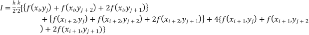
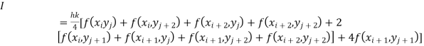
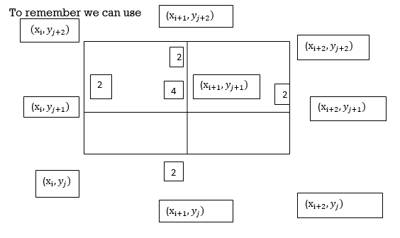
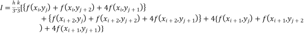
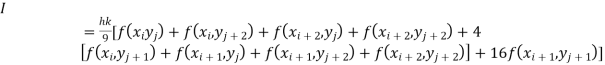
Simpson’s 1/3rd rule:
The double integration is defined by
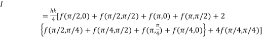
By Simpson’s 1/3 rd Rule

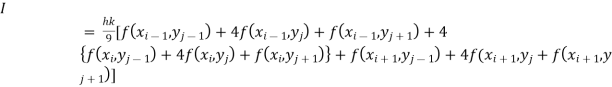
Also the double integration is defined by

Where .
.
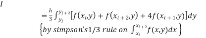
Again Applying Simpson’s 1/3 rd rule to each term with respect to y.
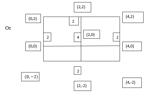
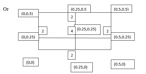
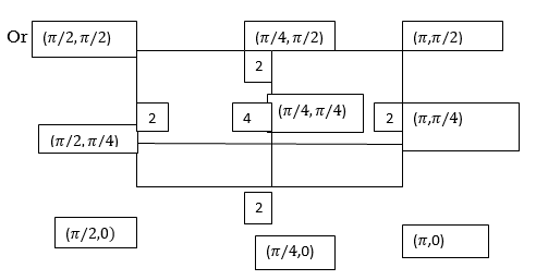
Example1: Evaluate 
Let 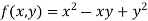
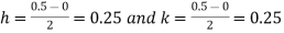
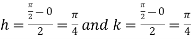
Here the interval of x and y are  and
and  .
.
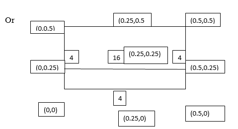
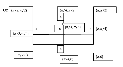
Let 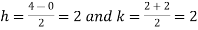
Consider the following table:
 |
 |
 |
 |
 |

|
 |
 |
 |
 |
 |
 |
 |
 |
 |
 |

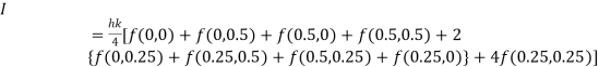
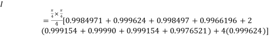
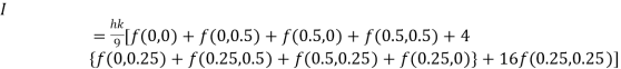
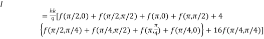
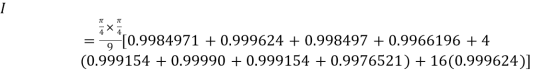
By Simpson’s 1/3 Rule


 .4444444
Example2: Evaluate 
Let 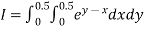
Here 
Let the number of interval be  .
.
 |
 |
 |
 |
 |

|
 |
 |
 |
 |
 |
 |
 |
 |
 |
 |
By Simpson’s 1/3 Rule


Example3: Evaluate 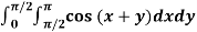
Let 
And 
 |
 |
 |
 |
 |
 |
 |
 |
 |
 |
 |
 |
 |
 |
 |
 |
By Simpson’s 1/3 Rule


Error in Integration
Error in Trapezoidal method
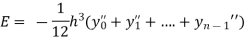
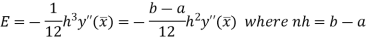
The total error in trapezoidal method is given by
Let  is the largest value of the n quantities on the right hand side of the above equation then
Error in Simpson’s Rule
The error in the Simpson’s rule is given by
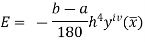
Where  is the largest value of the fourth derivative of y(x).
Error in Simpson’s 3/8 Rule
The error in this rule is given by
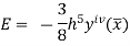
Where  is the largest value of the derivative of y(x).
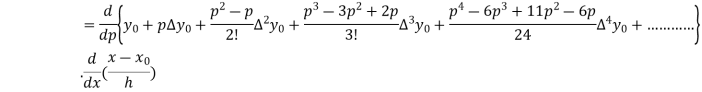
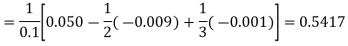
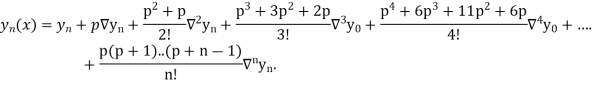
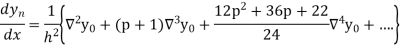
Newton’s forward Difference formula:
This method is useful for interpolation near the beginning of a set of tabular values.
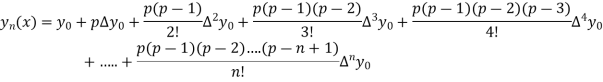
Where 
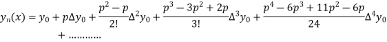
Differentiating both side with respect to p, we get

 h
h

This formula is applicable to compute the value of  for non tabular values of x.
For tabular values of x , we can get formula by putting 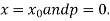
Therefore

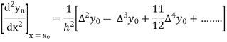
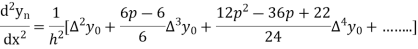
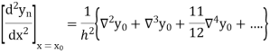
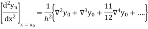
In similar manner we can get the formula for higher order by differentiating the previous order formulas

Again differentiating with respect to p, we get
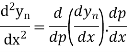

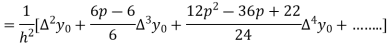
Hence

Also
And so on.
Example1: Given that
X | 1.0 | 1.1 | 1.2 | 1.3 |
Y | 0.841 | 0.891 | 0.932 | 0.963 |
Find  at
at  .
.
Here the first derivative is to be calculated at the beginning of the table, therefore forward difference formula will be used
Forward difference table is given below:
X | Y |  |  |  |
1.0
1.1
1.2
1.3 | 0.841
0.891
0.932
0.962 |
0.050
0.041
0.031 |
-0.009
-0.010 |
-0.001 |
By Newton’s forward differentiation formula for differentiation

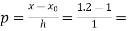
Here 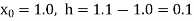
Example2: Find the first and second derivatives of the function given below at the point  :
:
X | 1 | 2 | 3 | 4 | 5 |
Y | 0 | 1 | 5 | 6 | 8 |
Here the point of the calculation  is at the beginning of the table,
Forward difference table is given by:
X | Y |  |  |  |  |
1
2
3
4
5 | 0
1
5
6
8 |
1
4
1
2 |
3
-3
1 |
-6
4
|
-10
|
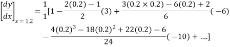
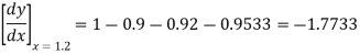
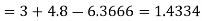
By Newton’s forward differentiation formula for differentiation
Here 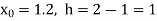 ,
,  0.
0.
Again
At 

Example3: From the following table of values of x and y find  for
for 
X | 1.00 | 1.05 | 1.10 | 1.15 | 1.20 | 1.25 | 1.30 |
Y | 1.0000 | 1.02470 | 1.04881 | 1.07238 | 1.09544 | 1.11803 | 1.14017 |
Here the value of the derivative is to be calculated at the beginning of the table.
Forward difference table is given by
X | Y |  |  |  |  |  |  |
1.00
1.05
1.10
1.15
1.20
1.25
1.30 | 1.0000
1.02470
1.04881
1.07238
1.09544
1.11803
1.14017 |
0.02470
0.02411
0.02357
0.02306
0.02259
0.02214 |
-0.00059
-0.00054
-0.00051
-0.00047
-0.00045 |
0.00005
0.00003
0.00004
0.00002 |
-0.00002
0.00001
-0.00002 |
0.00003
-0.00003 |
-0.00006 |
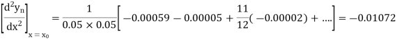
From Newton’s forward difference formula for differentiation we get


Here 

=0.48763
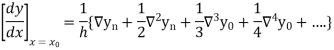
Newton Backward Difference Method:
This method is useful for interpolation near the ending of a set of tabular values.

Where 
Differentiating both side with respect to p, we get


This formula is applicable to compute the value of  for non tabular values of x.
For tabular values of x , we can get formula by putting 
Therefore

In similar manner we can get the formula for higher order by differentiating the previous order formulas

Differentiating both side with respect to p, we get


Also
Example1: Given that
X | 0.1 | 0.2 | 0.3 | 0..4 |
Y | 1.10517 | 1.22140 | 1.34986 | 1.49182 |
Find 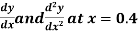 ?
?
Backward difference table:
X | Y |  |  |  |
0.1
0.2
0.3
0.4 | 1.10517
1.22140
1.34986
1.49182 |
0.11623
0.12846
0.14196 |
0.01223
0.01350 |
0.00127 |
Newton’s Backward formula for differentiation
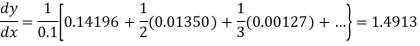
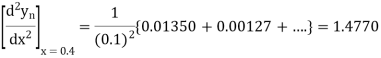
Here 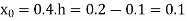
Example2: Given that
X | 1.0 | 1.2 | 1.4 | 1.6 | 1.8 | 2.0 |
Y | 0 | 0.128 | 0.544 | 1.296 | 2.432 | 4.0 |
Find the derivative of y at  ?
?
The difference table is given below:
X | Y |  |  |  |  |
1.0
1.2
1.4
1.6
1.8
2.0 | 0
0.128
0.544
1.296
2.432
4.0 |
0.128
0.416
0.752
0.136
1.568
|
0.288
0.336
0.384
0.432 |
0.048
0.048
0.048 |
0
0 |
Since the point  is at the beginning of the table therefore
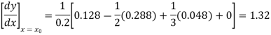
From Newton’s forward difference formula for differentiation we get
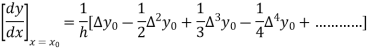
Here 
Since the point is at the end of the table therefore
Backward difference table is:
X | Y |  |  |  |  |
1.0
1.2
1.4
1.6
1.8
2.0 | 0
0.128
0.544
1.296
2.432
4.000 |
0.128
0.416
0.752
0.136
1.568 |
0.288
0.336
0.384
0.432 |
0.048
0.048
0.048 |
0
0 |
Newton’s Backward formula for differentiation

This method was first introduced by Lewis Fry Richardson. The applications of Richardson extrapolation includes Romberg integration, which applies Richardson extrapolation to the trapezoidal rule.
This is a sequence accelerated method. It is used to improve approximations of integrals.
Romberg integration:
This is a very powerful method, which uses the method of extrapolation.
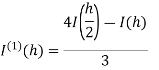
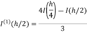
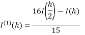
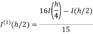
Romberg method for trapezium rule-
Step Length | Value of I  | Value of I  | Value of I  |


 | 

 | 
 |
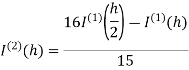 |
Here I denotes the exact value of integral and h, h/2, h/4 are the step lengths.
Note- Values at the end of each column are the most accurate.
Romberg method for Simpson’s 1/3 rule:
Step Length | Value of I  | Value of I  | Value of I  |


 | 

 | 
 |
 |
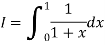
Example: Apply Romberg method for Simpson’s 1/3 rule to find the approximate value of the integral-
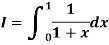
Sol.
Here we have-
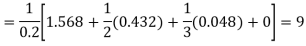
The approximations using the Simpson’s 1/3 rule to the integral with various values of the step lengths can be obtained as-

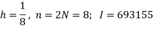
We have-

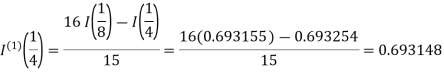
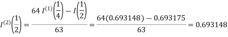
These results can be tabulated as-
Step length | Value of I  | Value of I  | Value of I  |
½
¼
1/8 | 0.694444
0.693254
0.693155 |
0.693175
0.693148 |
0.693148 |
Magnitude of the error is-
|I – 0.693148| = | 0.693147 – 0.693148| = 0.000001
References:
- E. Kreyszig, “Advanced Engineering Mathematics”, John Wiley & Sons, 2006.
- P. G. Hoel, S. C. Port and C. J. Stone, “Introduction to Probability Theory”, Universal Book Stall, 2003.
- S. Ross, “A First Course in Probability”, Pearson Education India, 2002.
- W. Feller, “An Introduction to Probability Theory and Its Applications”, Vol. 1, Wiley, 1968.
- N.P. Bali and M. Goyal, “A Text Book of Engineering Mathematics”, Laxmi Publications, 2010.
- B.S. Grewal, “Higher Engineering Mathematics”, Khanna Publishers, 2000.


