Unit - 2
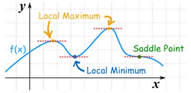
Extrema of functions of two variables
Let z = f (x, y) be a function of two independent variables x and y.
Definition of relative maximum and relative minimum-
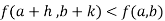
Relative maximum: f (x, y) is said to have a relative maximum at a point (a, b) if
f (a, b) > f (a + h, b + k)
For small positive or negative values of h and k i.e., f (a, b) the value of the function f at (a, b) is greater than the value of the function f at all points in some small neighbourhood of (a, b).
Relative minimum-
f (x, y) has a relative minimum at (a, b) if
f (a, b) < f (a + h, b + k).
Note-
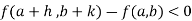
- f has a maximum at (a, b) if
 has the same negative sign for all small values of h, k; i.e.,
 < 0 a minimum at (a, b) if has the same positive sign, which means,
 > 0. Where
 = f (a + h, b + k) − f (a, b)
2. Extremum is a point which is either a maximum or minimum. The value of the function f at an extremum (maximum or minimum) point is known as the extremum (maximum or minimum) value of the function f.
3. Saddle point or minimax is a point where function is neither maximum nor minimum. At such point f is maximum in one direction while minimum in another direction.
Maxima and minima of function of two variables-
As we know that the value of a function at maximum point is called maximum value of a function. Similarly the value of a function at minimum point is called minimum value of a function.
The maxima and minima of a function is an extreme biggest and extreme smallest point of a function in a given range (interval) or entire region. Pierre de Fermat was the first mathematician to discover general method for calculating maxima and minima of a function. The maxima and minima are complement of each other.
Maxima and Minima of a function of one variables
If f(x) is a single valued function defined in a region R then
Maxima is a maximum point  if and only if
Minima is a minimum point  if and only if


Maxima and Minima of a function of two independent variables
Let  be a defined function of two independent variables.
Then the point  is said to be a maximum point of
  if
if
Or  =
= 
For all positive and negative values of h and k.
Similarly the point  is said to be a minimum point of
  if
if
Or  =
= 
For all positive and negative values of h and k.
Saddle point:
Critical points of a function of two variables are those points at which both partial derivatives of the function are zero. A critical point of a function of a single variable is either a local maximum, a local minimum, or neither. With functions of two variables there is a fourth possibility - a saddle point.
A point is a saddle point of a function of two variables if
![2 2 [ 2 ] 2
@f-= 0, @f--= 0, and @-f- @-f-- -@-f- < 0
@x @y @x2 @y2 @x @y](https://glossaread-contain.s3.ap-south-1.amazonaws.com/epub/1642647375_2325804.png)
At the point.
Stationary Value
The value  is said to be a stationary value of
  if
if
i.e. the function is a stationary at (a, b).
Rule to find the maximum and minimum values of 
- Calculate
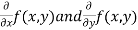 .
. - Form and solve
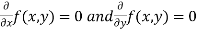 , we get the value of x and y let it be pairs of values
- Calculate the following values :
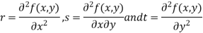
4. (a) If 
(b) If 
(c) If 
(d) If 
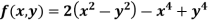
Example1 Find out the maxima and minima of the function
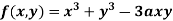
Sol:
Given 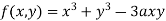 …(i)
…(i)
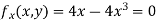
Partially differentiating (i) with respect to x we get
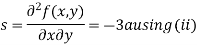
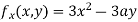 ….(ii)
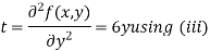
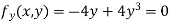
Partially differentiating (i) with respect to y we get
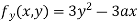 ….(iii)
Now, form the equations 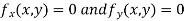
Using (ii) and (iii) we get


 using above two equations
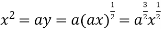
Squaring both side we get

Or 
This show that 
Also we get 
Thus we get the pair of value as 
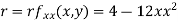
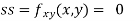
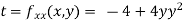
Now, we calculate
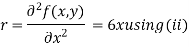
Putting above values in
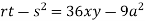
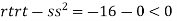
At point (0,0) we get
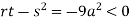
So, the point (0,0) is a saddle point.
At point  we get

So the point  is the minimum point where
In case 

So the point  is the maximum point where
Example2 Find the maximum and minimum point of the function
Partially differentiating given equation with respect to and x and y then equate them to zero
On solving above we get 
Also 
Thus we get the pair of values (0,0), ( ,0) and (0,
Now, we calculate
At the point (0,0)
So function has saddle point at (0,0).
At the point (

So the function has maxima at this point ( .
.
At the point (0,

So the function has minima at this point (0, .
.
At the point (
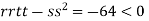
So the function has an saddle point at (
Key takeaways-
- The maxima and minima of a function is an extreme biggest and extreme smallest point of a function in a given range (interval) or entire region.
- If f(x) is a single valued function defined in a region R then
Maxima is a maximum point  if and only if
Minima is a minimum point  if and only if
3. A point is a saddle point of a function of two variables if
![2 2 [ 2 ] 2
@f-= 0, @f--= 0, and @-f- @-f-- -@-f- < 0
@x @y @x2 @y2 @x @y](https://glossaread-contain.s3.ap-south-1.amazonaws.com/epub/1642647379_2098217.png)
At the point.
Constrained optimization problems are problems for which a function f(x) is to be minimized or maximized subject to constraints.
Generally to calculate the stationary value of a function with some relation by converting the given function into the least possible independent variables and then solve them. When this method fail we use Lagrange’s method.
This method is used to calculate the stationary value of a function of several variables which are all not independent but are connected by some relation.
Let  be the function in the variable x, y and z which is connected by the relation
Rule:
a) Form the equation

Where  is a parameter.
b) Form the equation using partial differentiation is
(We always try to eliminate )
)
c) Solve the all above equation with the given relation 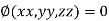
These give the value of 
These value obtained when substituted in the given function will give the stationary value of the function.
Example1 Divide 24 into three parts such that the continued product of the first, square of second and cube of third may be maximum.
Let first number be x, second be y and third be z.
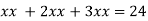
According to the question
Let the given function be 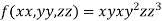
And the relation 
By Lagrange’s Method

 ….(i)
….(i)
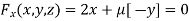
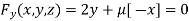
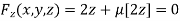
Partially differentiating (i) with respect to x,y and z and equate them to zero
 ….(ii)
 ….(iii)
 ….(iv)
From (ii),(iii) and (iv) we get

On solving

Putting it in given relation we get
Or 
Or 
Thus the first number is 4 second is 8 and third is 12
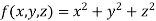
Example 2 The temperature T at any point  in space is
 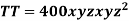 . Find the highest temperature on the surface of the unit sphere.
Given function is 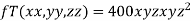
On the surface of unit sphere given  [
[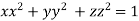 is an equation of unit sphere in 3 dimensional space]
By Lagrange’s Method

 ….(i)
….(i)
Partially differentiating (i) with respect to x, y and z and equate them to zero
 or
or 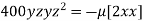 …(ii)
…(ii)
 or
or 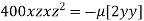 …(iii)
 …(iv)
…(iv)
Dividing (ii) and (ii) by (iv) we get

Using given relation 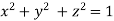
Or 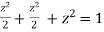
Or 
So that 
Or 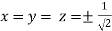
Thus points are 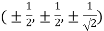
The maximum temperature is 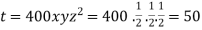
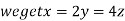
Example3 If  , Find the value of x and y for which
  is maximum.
Given function is 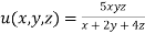
And relation is 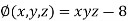
By Lagrange’s Method

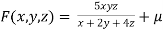 [
[ ] ..(i)
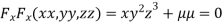
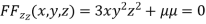
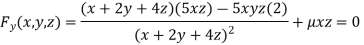
Partially differentiating (i) with respect to x, y and z and equate them to zero
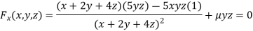
Or 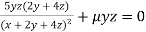 …(ii)
…(ii)
Or 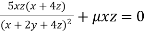 …(iii)
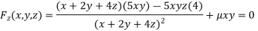
Or 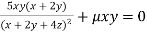 …(iv)
…(iv)
On solving (ii), (iii) and (iv) we get

Using the given relation we get 


So that 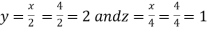
Thus the point for the maximum value of the given function is 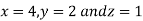
Example4 Find the points on the surface  nearest to the origin.
Let  be any point on the surface, then its distance from the origin
 is
is

Thus the given equation will be
And relation is 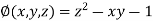
By Lagrange’s Method

 ….(i)
….(i)
Partially differentiating (i) with respect to x, y and z and equate them to zero
Or  …(ii)
…(ii)
Or  …(iii)
Or 
Or 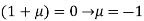
On solving equation (ii) by (iii) we get

And 
On subtracting we get 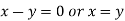
Putting in above 

Or 
Thus 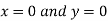
Using the given relation we get
 = 0.0 +1=1
Or 
Thus point on the surface nearest to the origin is 
Vector function-
Suppose  be a function of a scalar variable t, then-

Here vector  varies corresponding to the variation of a scalar variable t that its length and direction be known as value of t is given.
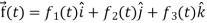
Any vector  can be expressed as-

Here  ,
,  ,
,  are the scalar functions of t.
Differentiation of a vector-
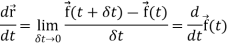
We can denote it as- 
Similarly  is the second order derivative of
Note-  gives the velocity and
  gives acceleration.
Note-
1. Velocity = 
2. Acceleration = 
The derivative of the velocity vector V(t) is called acceleration A(t), and it is given as-

Rules for differentiation-
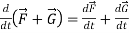
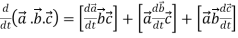
1. 
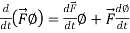
2. 
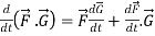
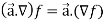
3. 
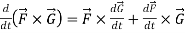
4. 
5. 
Example-1: A particle moves along the curve  , here ‘t’ is the time. Find its velocity and acceleration at t = 2.
Sol. Here we have-

Then, velocity

Velocity at t = 2,
= 
Acceleration = 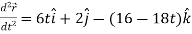
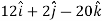
Acceleration at t = 2,
Example-2: If 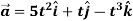 and
and 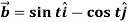 then find-
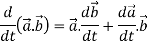
1. 
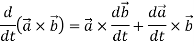
2. 
Sol. 1. We know that-


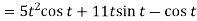
2.


Example-3: A particle is moving along the curve x = 4 cos t, y = 4 sin t, z = 6t. Then find the velocity and acceleration at time t = 0 and t = π/2.
And find the magnitudes of the velocity and acceleration at time t.
Sol. Suppose 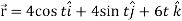
Now,
At t = 0 |   |
At t = π/2 |   |
At t = 0 | |v|=  |
At t = π/2 | |v|=  |
Again acceleration-
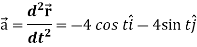
Now-
At t = 0 |  |
At t = π/2 |  |
At t = 0 | |a|=  |
At t = π/2 | |a|=  |
Scalar point function-
If for each point P of a region R, there corresponds a scalar denoted by f(P), in that case f is called scalar point function of the region R.
Note-
Scalar field- this is a region in space such that for every point P in this region, the scalar function ‘f’ associates a scalar f(P).
Vector point function-
If for each point P of a region R, then there corresponds a vector  then
then  is called a vector point function for the region R.
Vector field-
Vector filed is a reason in space such that with every point P in the region, the vector function  associates a vector
  (P).
(P).
Note-
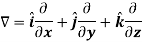
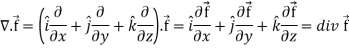
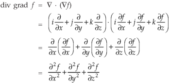
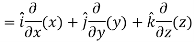
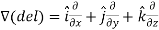
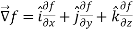
Del operator-
The del operated is defined as-
Example: Show that  where
where 
Sol. Here it is given-


= 
Therefore-
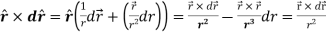 [Note-
Hence proved
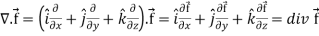
Divergence (Definition)-
Suppose  is a given continuous differentiable vector function then the divergence of this function can be defined as-
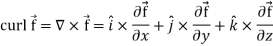
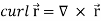
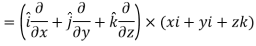
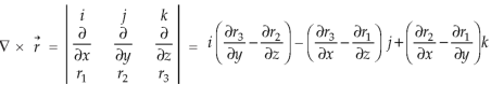
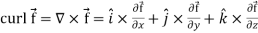
Curl (Definition)-
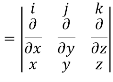
Curl of a vector function can be defined as-
Note- Irrotational vector-
If  then the vector is said to be irrotational.
Vector identities:
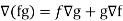
Identity-1: grad uv = u grad v + v grad u
Proof:
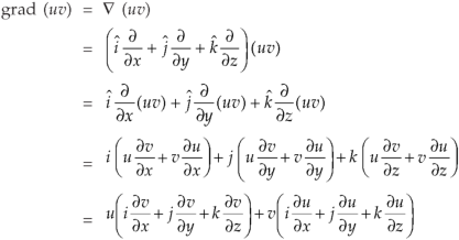
So that
Graduv = u grad v + v grad u
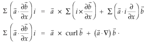
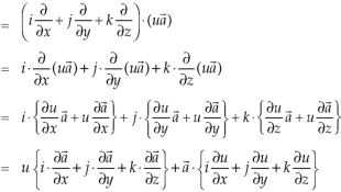
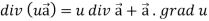
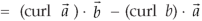
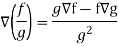
Identity-2: 
Proof:
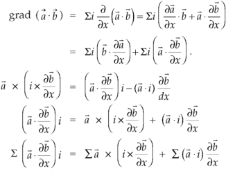
Interchanging  , we get-
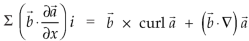
We get by using above equations-

Identity-3
Proof: 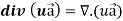
So that-
Identity-4
Proof:
So that,
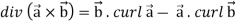
Identity-5: curl (u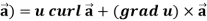
Proof:
So that
Curl (u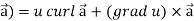
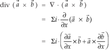
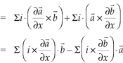
Identity-6: 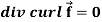
Proof:
So that-

Identity-7: 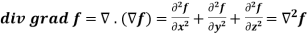
Proof:
So that-
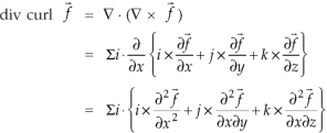
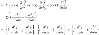
Example-1: Show that-
1. 
2.
Sol. We know that-

2. We know that-
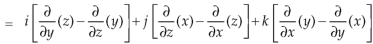
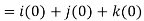 = 0
= 0
Example-2: If  then find the divergence and curl of
  .
.
Sol. We know that-
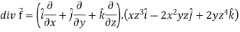
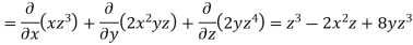
Now-
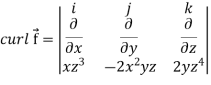
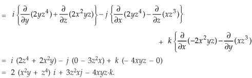
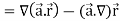
Example-3: Prove that 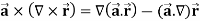
Note- here  is a constant vector and
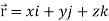
Sol. Here 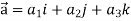 and
and 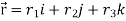
So that
Now-
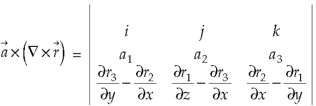
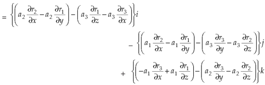
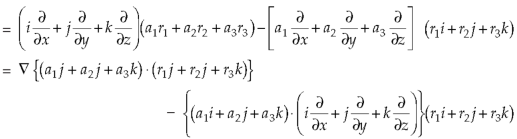
So that-
Key takeaways-
- Gradient of a constant (

If f and g are two scalar point functions, then
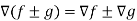
5. If f and g are two scalar point functions, then
6. If f and g are two scalar point functions, then-
7. 
8. 
9. If  then the vector is said to be irrotational.
10. grad uv = u grad v + v grad u
11. 
12. curl (u
13. Any vector  can be expressed as-
Here  ,
,  ,
,  are the scalar functions of t.
1. Velocity = 
2. Acceleration = 
3. Scalar field- this is a region in space such that for every point P in this region, the scalar function ‘f’ associates a scalar f(P).
4. Vector field-
Vector filed is a reason in space such that with every point P in the region, the vector function  associates a vector
  (P).
(P).
Double Integral over Rectangular and general regions
Consider a function f (x, y) defined in the finite region R of the x-y plane. Divide R into n elementary areas A1, A2,…,An. Let (xr, yr) be any point within the rth elementary are Ar
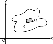
f (x, y) dA = f (xr, yr) A
Evaluation of Double Integral when limits of Integration are given(Cartesian Form).
Ex-1: Evaluate

Sol:
Given
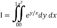
Here limits of inner integral are functions of y therefore integrate w.r.t y,
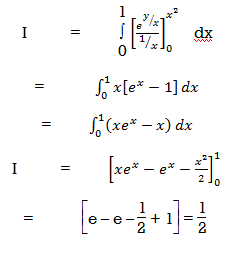
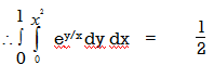
Ex-2: Evaluate
Sol:
Given:
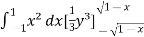
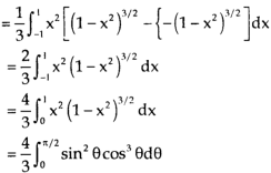
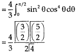
Here the limits of inner integration are functions of y therefore first integrate w.r.t y.
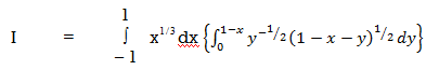
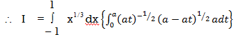
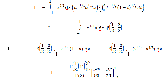
Put 1 – x = a (constant for inner integral)
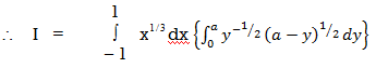
Put y = at dy = a dt
y | 0 | a |
t | 0 | 1 |
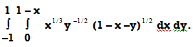
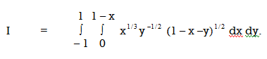
Ex-3: Evaluate
Sol:
Let,
Here limits for both x and y are constants, the integral can be evaluated first w.r.t any of the variables x or y.
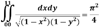
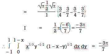
Ex-4: Evaluate
Sol:
Let
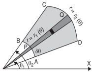
In polar coordinates, we need to evaluate
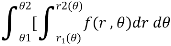
Over the region bounded by θ1 and θ2.
And the curves r1(θ) and r2(θ)
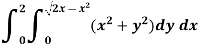
Example-1: Evaluate the following by changing to polar coordinates,
Sol. In this problem, the limits for y are 0 to  and the limits for are 0 to 2.
Suppose,
y = 
Squaring both sides,
y² = 2x - x²
x² + y² = 2x
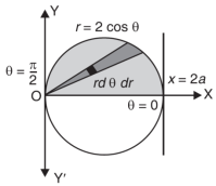
But in polar coordinates,
We have,
r² = 2r cosθ
r = 2 cosθ
From the region of integration, r lies from 0 to 2 cosθ and θ varies from 0 to π / 2.
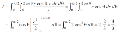
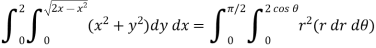
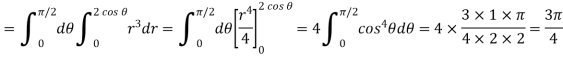
As we know in case of polar coordinates,
Replace x by r cosθ and y by r sinθ, dy dx by r drdθ,
We get,
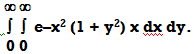
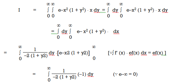
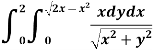
Example-2: Evaluate the following integral by converting into polar coordinates.
Sol.
Here limits of y,
y = 
y² = 2x - x²
x² + y² = 2x
x² + y² - 2x = 0 ………………(1)
Eq. (1) represent a circle whose radius is 1 and centre is ( 1, 0)
Lower limit of y is zero.
Region of integration in upper half circle,
First we will convert into polar coordinates,
By putting
x by r cos θ and y by r sinθ, dy dx by r drdθ,
Limits of r are 0 to 2 cosθ and limits of θ are from 0 to π / 2.
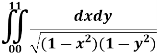
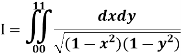
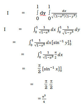
Example-3: Evaluate 
Sol. Let the integral,
I = 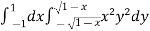
=
Put x = sinθ
= π / 24 ans.
Key takeaways:
In polar coordinates, we need to evaluate

Over the region bounded by θ1 and θ2.
References:
1. S C Mallik and S Arora: Mathematical Analysis, New Age International.
2. Publications S Ghorpade, B V Limaye, Multivariable calculus, Springer international edition.
3. Higher engineering mathematic, Dr. B.S. Grewal, Khanna publishers.
4. Advanced engineering mathematics, by HK Dass.
5. Erwin Kreyszig, Advanced Engineering Mathematics, 9thEdition, John Wiley & Sons, 2006.


