Unit - 3
Transportation problem and its mathematical formulation
The transportation algorithms help to minimize the total cost of transporting a homogeneous commodity (product) from supply centres to demand centres. However, it can also be applied to the maximization of total value or utility.
The structure of transportation problem involves a large number of shipping routes from several supply centres to several demand centres. Thus, objective is to determine shipping routes between supply centres and demand centres in order to satisfy the required quantity of goods or services at each destination centre, with available quantity of goods or services at each supply centre at the minimum transportation cost and/ or time.
General Mathematical Model of Transportation Problem
Let there be m sources of supply, S1, S2, . . ., Sm having ai (i = 1, 2, . . ., m) units of supply (or capacity), respectively to be transported to n destinations, D1, D2, . . ., Dn with bj ( j = 1, 2, . . ., n) units of demand (or requirement), respectively. Let cij be the cost of shipping one unit of the commodity from source i to destination j. If xij represents number of units shipped from source i to destination j, the problem is to determine the transportation schedule so as to minimize the total transportation cost while satisfying the supply and demand conditions. Mathematically, the transportation problem, in general, may be stated as follows:

Subject to the constraints


And

Simple Formulation of Transportation Problems
Let a manufacturer of an item has m origin situated at places O1, O2, . . ., Oi, . . ., Om and let there are n destinations at D1, D2, . . . Dj . . . Dn. The aggregate of the capacities of all m origins is assumed to be equal to the aggregate of the requirements of all n destinations. Let Cij be the cost of transporting one unit from origin i to destination j. Let ai be the capacity/availability of items at origin i and bj, the requirement/demand of the destination j.
Then this transportation problem can be expressed in a tabular form as given below-
Origin | Destinations     | Capacity |
  . . .
 . . .  |         . . .
    . . .     |   . . .  . .
.  |
Requirement |     | Total |
For the existence of a feasible solution to a transportation problem is given as

This equation define that the total requirement equals the total capacity. If it is not so, a dummy origin or destination is created to balance the total capacity and requirement.
Let xij be the number of units to be transported from origin i to destination j and Cij the corresponding cost of transportation. Then the total transportation cost is  .
.
This means that the product of the number of units allocated to each cell with the transportation cost per unit for that cell is calculated and added for all cells. Our objective is to allocate the units in such a way that the total transportation cost is least. The problem can also be stated as a linear programming problem as follows:
We are to minimise the total transportation cost-

Subject to the constraints-


And

For all i = 1,2, ...., m and j = 1,2, ......n.
This problem can be solved by the simplex method but it is very lengthy so that we use an alternative method which is the ‘transportation method’.
Solution by transportation method involves making a transportation model in the form of a matrix, finding an initial basic feasible solution, performing optimality test and moving towards an optimal solution.
Note- When total demand equals total supply, the transportation problem is said to be balanced.
Key takeaways:
- When the total supply is equal to the total demand, the problem is called a balanced transportation problem, otherwise it is called an unbalanced transportation problem. The unbalanced transportation problem can be made balanced by adding a dummy supply centre (row) or a dummy demand centre (column) as the need arises.
- When the number of positive allocations (values of decision variables) at any stage of the feasible solution is less than the required number (rows + columns – 1), i.e. number of independent constraint equations, the solution is said to be degenerate, otherwise non-degenerate. For proof, see Appendix at the end of this chapter.
- Cells in the transportation table having positive allocation, i.e., xij > 0 are called occupied cells, otherwise are known as non-occupied (or empty) cells.
North West Corner Rule (NWCR)
1. Select the North-west (i.e., upper left) corner cell of the table and allocate the maximum possible units between the supply and demand requirements. During allocation, the transportation cost is completely discarded (not taken into consideration).
2. Delete that row or column which has no values (fully exhausted) for supply or demand.
3. Now, with the new reduced table, again select the North-west corner cell and allocate the available values.
4. Repeat steps (2) and (3) until all the supply and demand values are zero.
5. Obtain the initial basic feasible solution.
Example: Find out the initial feasible solution for transportation cost involved in the problem shown in table:

Sol:

As under the process of NWC method, we allocate  = 20. Now demand for the first column is satisfied, therefore, eliminate that column.
Proceeding in this way, we observe that

Delete the row if supply is exhausted.
Delete the column if demand is satisfied.
Here, number of retail shops (n) = 4, and
Number of factories (m) = 3
Number of basic variables = m + n – 1 = 3 + 4 – 1 = 6.
Initial basic feasible solution:
20 × 3 + 20 × 5 + 10 × 7 + 40 × 8 + 35 × 2 + 25 × 2 = 670
Least Cost Method (LCM)
There are several methods available to get the first basic viable solution to your shipping problem. Only the following three are discussed here. To find the first basic viable solution, the total supply should be equal to the total demand.
Method: Least common multiple method (LCM)
The lowest cost method is more economical than the northwest corner rule because it starts with a low starting cost. The various steps involved in this method are summarized below.
Step 1: Find the cell with the lowest (minimum) cost in the transport table.
Step 2: Assign the maximum amount that can be executed in this cell.
Step: 3: Delete the row or column to which the assignment will be made.
Step: 4: Repeat the above steps for the reduced transport table until all allocations are complete.
Example
Use the lowest cost method to get the first basic viable solution to the next shipping problem.
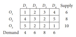
Here, Oi and Dj indicate the i-th starting point and the j-th destination, respectively.
Solution:
Total supply = total demand = 24
The problem given is a balanced transportation problem.
Therefore, there is a viable solution to the given problem.
The transportation issues given are:
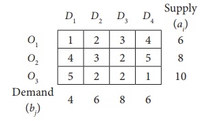
The minimum cost is 1, which corresponds to cells (O1, D1) and (O3, D4).
Get cells (O1, D1) arbitrarily.
Allocate min (6,4) = 4 units in this cell.
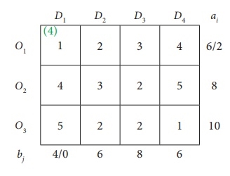
The shrunk table
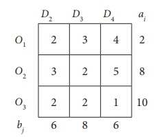
The lowest cost corresponds to the cell (O3, D4). Allocate a minimum (10,6) = 6 units to this cell.
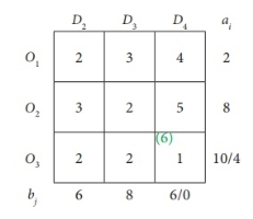
The shrunk table
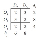
Minimum cost 2 corresponds to cells (O1, D2), (O2, D3), (O3, D2), (O3, D3).
Allocate min (2,6) = 2 units to this cell.
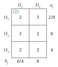
The shrunk table
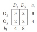
The minimum cost is 2, which corresponds to cells (O2, D3), (O3, D2), (O3, D3).
Allocate a minimum (8,8) = 8 units to this cell.
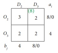
The shrunk table

Here we assign 4 units to the cell (O3, D2)
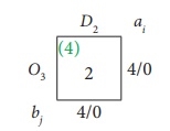
Therefore, it has the following assignments:
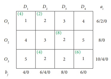
Transport schedule:
O1 → D1, O1 → D2, O2 → D3, O3 → D2, O3 → D4
Total shipping cost
= (4 × 1) + (2 × 2) + (8 × 2) + (4 × 2) + (6 × 1)
= 4 + 4 + 16 + 8 + 6
= Rs. 38.
Example
Use the lowest cost method to determine the quantity that needs to be stepped from the factory to different destinations for the next shipping problem:
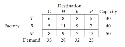
The cost is expressed in rupees per unit shipped.
Solution:
Total capacity = total demand
The problem given is a balanced transportation problem.
Therefore, there is a viable solution to the given problem.
Given the transportation problem
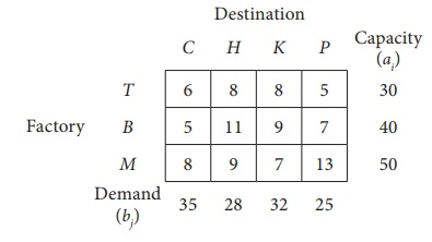
First assignment:
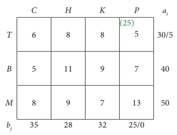
Second assignment:
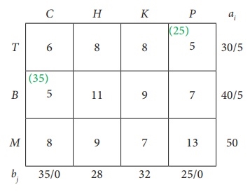
Third assignment:
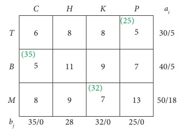
Fourth assignment:
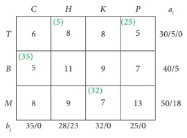
Fifth assignment:

6th assignment:
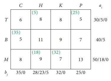
Transport schedule:
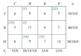
T → H, T → P, B → C, B → H, M → H, M → K
Total shipping cost = (5 × 8) + (25 × 5) + (35 × 5) + (5 × 11) + (18 × 9) + (32 × 7)
= 40 + 125 + 175 + 55 + 162 + 224
= £ 781
Vogel’s Approximation Method (VAM)
This method has the following steps-
- For each row of the transportation table, we identify the least and second least costs. We find the difference between these two and display it to the right of that row in a new column formed by extending the table on the right. Likewise, we find such differences for each column and display it below that column in a new row formed for the purpose by extending the table at the bottom. The new column and row formed by extending the table at the right and bottom are labelled as penalty column and penalty row, respectively. If two cells in a row (or column) contain the same least costs then the difference is taken as zero.
- From amongst these difference values displayed in the penalty column and the penalty row, we select the largest value (largest difference). We, allocate the maximum possible units to the least cost cell in the selected column or row. If a tie occurs amongst the largest differences, the choice may be made for that row or column, which has the least cost. In case there is a tie in such least cost as well, choice may be made from that row or column by which maximum requirements are exhausted. The cell so chosen is allocated the units and the corresponding exhausted row (or column) is removed (or ignored) from further consideration.
- We compute the column and row differences for the reduced transportation table and repeat the procedure until all column and row totals are exhausted.
Note- This method is also called the penalty method.
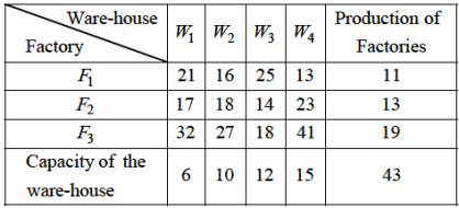
Example: Find the initial Basic feasible solution of the following transportation problem by Vogel’s apprx. Method.
Sol.
Step-1: Here, the total production of the factories and total capacities of the ware-houses being the same i.e. 43, the problem is balanced.
Step-2: Initial Basic Feasible solution- By VAM the difference between the smallest and next to the smallest costs in each row and each column are computed and written within brackets against the respective rows and column of table 1.

From table-1,
Largest difference (10) corresponds to 4th column. In this column, first row corresponds to lowest cost (13). So allocate to (1, 4) box with min (11, 23) ie 11.
The first row is exhausted. The reduced table 1 is written below

From table-2,
Largest difference 18 corresponds to 4th column. In this column first row corresponds to the lowest cost (13). So allocate to (1, 4) box min (4, 13) i.e. 4.
Fourth column is exhausted. The reduced table is written below

From table 3, largest difference (15) corresponds to first column. In this column first row corresponds to the lowest cost (17). So allocate to the (1, 1) box with the min (6, 9) ie 6.
First column of table - 3 is exhausted and the reduced table 4 is written below.

The largest difference (9) occurs at two places. So there is a tie here. Costs on both largest differences are identical choose any one. Allocate (1, 1) box with min (3, 10) i.e. 3.
First row of table-4 is exhausted. The reduced table 4 is written below:
From table 5, largest difference (27) corresponds to first column and is written in the box of first column and first row.
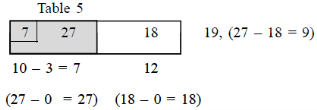
First column of table 5 is exhausted. The reduced table 6 has only one box.
From table 6, minimum of 12 and 12 is 12 and is written in this box.

The initial basic feasible solution is given in the table below-

Note- The initial solution obtained by any of the three methods must satisfy the following conditions.
1. The solution must be feasible, i.e., the supply and demand constraints must be satisfied (also known as rim conditions).
2. The number of positive allocations, N must be equal to m + n – 1, where m is the number of rows and n is the number of columns.
Note-
Balanced Transportation Problem: when the total supplies of all the sources are equal to the
Total demand of all destinations.
Basic Feasible Solution: A feasible solution to an 'm' origin and 'n; destination is said to be basic, if the number of positive allocations are (m+n+1).
Degeneracy: When the number of filled cells is less than the number of rows plus the number of columns minus one.
Practice questions
Q1: Find the initial basic feasible solution for the transportation problem given in following table.

Q2: A computer manufacturer has decided to launch an advertising campaign on television, magazines and radio. It is estimated that maximum exposure for these media will be 70, 50, and 40 million respectively. According to a market survey, it was found that the minimum desired exposures within age groups 15-20, 21-25, 26-30, 31-35 and above 35 are 10, 20, 25, 35 and 55 million respectively. The table below gives the estimated cost in paise per exposure for each of the media. Determine an advertising plan to minimize the cost.

Key takeaways:
- A transportation problem basically deals with that problem which aims to find the best way to fulfill the demand of various demand sources using the capacities of various supply points.
- The transportation problem applies to situations where a single commodity is to be transported from various sources of supply (origins) to various demands (destinations).
- Constraints: In transportation problems, there are supply constraints for each source, and demand constraints for each destination.
- Transportation problems are often used in, surprise, transportation planning. But it should always be remembered that the transportation problem is only a special topic of the linear programming problems.
- Balanced Transportation Problem: when the total supplies of all the sources are equal to the total demand of all destinations.
- Basic Feasible Solution: A feasible solution to an 'm' origin and 'n; destination is said to be basic, if the number of positive allocations are (m+n+1).
- Degeneracy: When the number of filled cells is less than the number of rows plus the number of columns minus one.
The algorithm for solving a transportation problem may be summarized into the following steps:
Step 1:
Formulate the problem and arrange the data in the matrix form The formulation of the transportation problem is similar to the LP problem formulation. In transportation problem, the objective function is the total transportation cost and the constraints are the amount of supply and demand available at each source and destination, respectively.
Step 2:
Obtain an initial basic feasible solution In this chapter, following three different methods are discussed to obtain an initial solution:
• North-West Corner Method,
• Least Cost Method, and
• Vogel’s Approximation (or Penalty) Method.
The initial solution obtained by any of the three methods must satisfy the following conditions:
(i) The solution must be feasible, i.e. it must satisfy all the supply and demand constraints (also called rim conditions).
(ii) The number of positive allocations must be equal to m + n – 1, where m is the number of rows and n is the number of columns.
Any solution that satisfies the above conditions is called non-degenerate basic feasible solution, otherwise, degenerate solution.
Step 3:
Test the initial solution for optimality In this chapter, the Modified Distribution (MODI) method is discussed to test the optimality of the solution obtained in Step 2. If the current solution is optimal, then stop. Otherwise, determine a new improved solution.
Step 4:
Updating the solution Repeat Step 3 until an optimal solution is reached.
Overview
When one task is to be assigned to one person in such a way that the total person hours are minimized, then this kind of problem is known as assignment problem.
Assignment problems are the special case of transportation problems. In assignment problems the number of sources and destinations are same.
Allocation problems are a special sort of applied mathematics problem that handles the one-to-one allocation of various resources to different activities. It does it during a way that minimizes the value or time involved within the process and maximizes profits or sales. The issues are often solved by the simplex or transport method, but the allocation model provides an easier approach to those problems.
At the factory, supervisors have access to six workers and may dismiss 6 jobs. He will need to make a choice on which job should tend to which worker. The matter forms a one-to-one foundation. This is often a matter of allocation.
Formulation of cost matrix
Let there are n persons and n jobs and the assignment of jobs has to be done on a one-to-one basis. We can state this assignment problem in the form of an n×n matrix of real numbers which is called cost matrix.
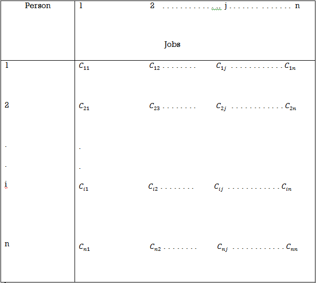
Here  is the amount of time taken by i’th person to complete jth job.
Suppose  denotes the jth job assigned to the ith person.
Then the mathematical representation of assignment problem will be as follows

Where i = 1,2,…,n and j = 1,2,..,m
Subject to

Mathematical formulation:
The basic viable solution to the allocation problem cons
Ists of (2n – 1) variables, where the (n – 1) variable is zero and n is that the number of jobs or facilities. Thanks to this high degree of degeneracy, solving problems with normal shipping methods are often a posh and time-consuming task. Therefore, another method springs . It's vital to formulate the matter before proceeding to absolutely the law.
Suppose xjj may be a variable defined as follows:
If the primary job is assigned to the jth machine or facility
0 if the i-th job isn't assigned to the j-th machine or facility.
Therefore,


Here, the matter is made one-to-one, or one job is assigned to at least one facility or machine.
The total allocation cost is

The above definition is often evolved into a mathematical model as follows:
Determine xij> 0 (i, j = 1,2,3… n),
Minimize,

Be constrained


Xij is either 0 or 1.
 - indicates the cost of assigning ith job to jth individual or vice versa, Viij = 1 to n.
 - indicates whether ith job is assigned to jth person or not.
 if ith job is assigned to jth person ‘0’ otherwise.
Application of Assignment Problem
1. Assignment of employees to machines.
2. Assignment of operators to jobs.
3. Effectiveness of teachers and subjects.
4. Allocation of machines for optimum utilization of space.
5. Allocation of salesmen to different sales areas.
6. Allocation of clerks to various counters.
Types of Assignment Problem
The assignment problems are of two types. It can be either
(i) Balanced or
(ii) Unbalanced.
If the number of rows is equal to the number of columns or if the given problem is a square matrix, the problem is termed as a balanced assignment problem. If the given problem is not a square matrix, the problem is termed as an unbalanced assignment problem.
Note- Assignment Problem is a variation of the transportation problem with two characteristics:
1. Cost matrix is a square matrix
2. The optimal solution for the problem would always be such that there would be only one assignment in a given row or column of the cost matrix
Initial basic feasible solution can be found out by following:
1. Reduction Theorem
2. Hungarian method
Reduction Theorem can be used for solving assignment problems with an objective of minimization of costs. For such maximization assignment problems, commonly used rules are:
1. Blind fold assignment/assignment by intuition.
2. Converting the maximization problem into minimization by considering the largest element in the whole matrix.
3. Converting the maximization problem into minimization by using negative signs for all the elements in the profit matrix.
Example: Solve the following assignment problem and find the minimum cost.

Sol:
Here we will use reduction rules,
Step 1: Row-wise Reduction of the matrix.

Step 2: Column-wise Reduction of the matrix.

Step 3: Assignment of jobs to workers.

Step 4: Calculation of the Minimum total job cost associated with the assignment.

The minimum total cost required to complete the assignment is Rs. 38.
Key takeaways:
1. Assignment Problem is a variation of the transportation problem with two characteristics:
(a) Cost matrix is a square matrix
(b) The optimal solution for the problem would always be such that there would be only one assignment in a given row or column of the cost matrix
2. An assignment problem seeks to minimize the total cost assignment of n workers to n jobs.
3. An assignment problem is a special case of a transportation problem in which all supplies and all demands are equal to 1; hence assignment problems may be solved as linear programs.
Consider a minimization type objective function. Resolving this allocation issue involves the subsequent steps:
1. Find the littlest cost element in each row of the required cost table, starting with the primary row. Here, this smallest element is subtracted from each element therein row. Therefore, get a minimum of one zero in each row of this new table.
2. After creating the table (as in step 1), get the columns of the table. Start with the primary column and find rock bottom cost think about each column. Then subtract this smallest element from each element therein column. After performing steps 1 and a couple of, you'll see a minimum of one zero in each column of the reduced cost table.
3. The reduced table is now allocated within the following way:
(I) Rows are continuously inspected until a row with just one zero is found. This assignment to one zero is formed by placing a square □ around it, with all other zeros being strikethrough (x) within the corresponding column. This is often because they're not used for other assignments during this column. The steps are performed for every row.
(ii) Step 3 (i) am performed on the column as follows: -Columns are continuously inspected until a column with just one zero is found. Now, by placing a square around it, this single zero is assigned, and at an equivalent time all other zeros within the corresponding row are erased (x) A step is performed on each column. I will.
(iii) Steps 3, (i), and three (ii) are repeated until all zeros are marked or strikethrough is drawn. Here, if the amount of zeros marked or the amount of allocations made is adequate to the amount of rows or columns, the simplest solution is achieved. There’s exactly one assignment for every column or column, with none assignment. During this case, attend step 4.
4. At this stage, draw the minimum number of lines (horizontal and vertical) needed to hide all the zeros within the matrix obtained in step 3. Use the subsequent procedure.
(i) Put a check on all unassigned lines.
(ii) Now mark of these columns that have zeros within the graduated rows (iii) Now check all rows that haven't yet been marked and are assigned to the marked columns.
(iv) All steps, namely (4 (i), 4 (ii), 4 (iii), are repeated until no row or column are often marked.
(v) Draw a line through all unmarked rows and marked columns. Also note that in an n x n matrix, lines but "n" always cover all zeros if there's no solution between them.
5. In step 4, the amount of lines drawn is n or the number of lines, it's the best solution. If not, go to step 6.
6. Select the smallest element from all uncovered elements. Here, this element is subtracted from all uncovered elements and added to the element at the intersection of the two lines. This is the new allocation matrix.
7. Repeat step (3) until the number of allocations is equal to the number of rows or columns.
Maximization & Minimization Type Problems
For maximizing allocation problems
There may be situations where allocation issues require maximization of profits.
Such a problem can be solved by transforming a given maximization problem into a minimization problem by subtracting all the elements of a given matrix from the highest elements.
Example
Find a solution to the allocation problem using the Hungarian method (for MAX)
Job | I | II | III | IV |
A | 42 | 35 | 28 | 21 |
B | 30 | 25 | 20 | 15 |
C | 30 | 25 | 20 | 15 |
D | 24 | 20 | 16 | 12 |
Solution:
Number of rows = 4 and number of columns = 4
The problem here is the Maximization type, which translates to minimization by subtracting from the maximum value of 42.
| |||||
| II | III | IV |
| |
A | 42 | 35 | 28 | 21 |
|
B | 30 | 25 | 20 | 15 |
|
C | 30 | 25 | 20 | 15 |
|
D | 24 | 20 | 16 | 12 |
|
|
|
|
|
|
|
The issues given here are balanced.
Step-1: Find the smallest element in each row and subtract from that row
I | II | III | IV |
| |
A | 0 0=0-0 | 7 7=7-0 | 14 14=14-0 | 21 21=21-0 | (-0) Minimum element of 1st row |
B | 0 0=12-12 | 5 5=17-12 | 10 10=22-12 | 15 15=27-12 | (-12) Minimum element of 2nd row |
C | 0 0=12-12 | 5 5=17-12 | 10 10=22-12 | 15 15=27-12 | (-12) Minimum element of 3rd row |
D | 0 0=18-18 | 4 4=22-18 | 8 8=26-18 | 12 12=30-18 | (- |
Step-2: Find the smallest element in each column and subtract from that column.
| I | II | III | IV |
|
A | 0 0=0-0 | 3 3=7-4 | 6 6=14-8 | 9 9=21-12 |
|
B | 0 0=0-0 | 1 1=5-4 | 2 2=10-8 | 3 3=15-12 |
|
C | 0 0=0-0 | 1 1=5-4 | 2 2=10-8 | 3 3=15-12 |
|
D | 0 0=0-0 | 0 0=4-4 | 0 0=8-8 | 0 0=12-12 |
|
| (-0) Minimum element of 1st column | (-4) Minimum element of 2nd column | (-8) Minimum element of 3rd column | (-12) |
|
Step-3: Make an allocation in the opportunity cost table
(1) Since the cells in the row direction (A, I) are assigned, the cells in the column direction (B, I), (C, I), and (D, I) intersect.
(2) Since the cells (D, II) in the column direction are assigned, the cells (D, III) and (D, IV) in the row direction intersect.
Row and column orientations shown in the table
| |||||
I | II | III | IV |
| |
A | [0] (1) Rowwise cell (A,I) is assigned | 3 | 6 | 9 |
|
B | 0 Column wise (B,I) crossed off because | 1 | 2 | 3 |
|
C | 0 Column wise (C,I) crossed off because | 1 | 2 | 3 |
|
D | 0 Columnwise (D,I) crossed off because | [0] (2) Columnwise cell (D,II) is assigned | 0 Rowwise (D,III) crossed off because | 0 Rowwise (D,IV) crossed off because |
|
|
|
|
|
|
|
Step-4: Number of allocations = 2, Number of rows = 4
The solution is not optimal because this is not equal.
Step-5: Cover 0 with minimum number of rows
(1) Since there is no assignment in line B, mark (✓) line B
(2) Since there is no assignment, mark line C (✓).
(3) Mark (✓) column I because column B in row B is 0.
(4) Mark (✓) row A because column I has an assignment for this row A.
(5) Draw a straight line through unmarked row D and marked column I because no other row or column can be marked.
Check unassigned rows and assigned columns
| |||||
II | III | IV |
| ||
A | [0] | 3 | 6 | 9 | ✓(4) (4) Mark(✓) row A since column I has an assignment in this row A. |
B | 0 | 1 | 2 | 3 | ✓(1) (1) Mark(✓) row B since it has no assignment |
C | 0 | 1 | 2 | 3 | ✓(2) (2) Mark(✓) row C since it has no assignment |
D | 0 | [0] | 0 | 0 |
|
| ✓ |
|
|
|
|
Step-6: Create a new revised table by selecting the smallest element from cells that are not covered by any line (eg k = 1).
Subtract k = 1 from all the elements in the cell that are not covered by the line.
Add k = 1 to all elements of the intersection cell of the two lines.
| |||||
I | II | III | IV |
| |
A | 0 cell covered by a line | 2 2=3-1 | 5 5=6-1 | 8 8=9-1 |
|
B | 0 cell covered by a line | 0 0=1-1 | 1 1=2-1 | 2 2=3-1 |
|
C | 0 cell covered by a line | 0 0=1-1 | 1 1=2-1 | 2 2=3-1 |
|
D | 1 1=0+1 | 0 cell covered by a line | 0 cell covered by a line | 0 cell covered by a line |
|
|
|
|
|
|
|
|
|
|
|
|
|
Repeat steps 3-6 until you get the best solution.
Step-3: Make an allocation in the opportunity cost table
(1) Since the cells in the row direction (A, I) are assigned, the cells (B, I) and (C, I) in the column direction intersect.
(2) Since the cells in the row direction (B, II) are assigned, the cells (C, II) and (D, II) in the column direction intersect.
(3) Since the cells in the column direction (D, III) are assigned, the cells in the row direction (D, IV) intersect.
Case study
Example: A company has taken the third floor of a multi-storied building for rent to locate one of its zonal offices. There are five main rooms in this floor to be assigned to five managers. Each room has its own advantages and disadvantages. Some have two cupboards, some are closer to the washrooms or to the canteens, some are of big sizes and are on different floors, etc. Each of the five managers were asked to rank their room preferences amongst the rooms 201, 302, 103, 304 and 205. Their preferences were recorded in a table as indicated below:
Manager
     302 302 103 302 201 103 304 201 205 302 Rooms 304 205 304 304 304 201 205 103 302 |
Most of the managers did not include all five rooms in the list since they were not satisfied with some of them. Assuming that their preferences can be quantified by numbers, find out which manager should be assigned which room so that their total preference ranking is minimum.
Sol. Here we will give the ranks 1, 2, 3, 4 and 5 to the first, second, third, fourth and fifth preferences. We assign to the cells for which no preference is given. Thus, the given problem can be represented by the following assignment table given below-
| 201 | 302 | 103 | 304 | 205 |
 |  | 1 | 2 | 3 |  |
 | 4 | 1 |  | 2 | 3 |
 | 2 | 5 | 1 | 3 | 4 |
 |  | 1 | 4 | 3 | 2 |
 | 1 | 2 |  | 3 |  |
And then by using the Hungarian method, we get-

Since each row and each column has one and only one assigned zero, the optimum assignment,
The assignment with maximum satisfaction is made and is given by:

Simple Formulation of Assignment Problems:
Meaning of allocation problem:
Allocation problems are specific cases of transportation problems where the goal is to allocate an outsized number of resources to an equivalent number of activities so as to attenuate the entire cost or maximize the entire profit of the allocation.
Allocation issues arise because available resources like men, machines, etc. have different degrees of efficiency for performing different activities. Therefore, there are different costs, benefits, or losses to perform different activities.
Definition of assignment problem:
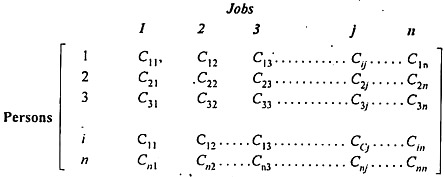
Suppose you've got n jobs to run and n people can run these jobs. Efficiency varies, but assumes that every person can run each job in just one occasion period. However, if the i-th person is assigned to the j-th job, cij are going to be the value. The matter is finding an assignment (which job should be assigned to which person on a one-to-one basis). This sort of problem is understood as an allocation problem in order that the entire cost of running all jobs is minimized.
Assignment issues are often expressed within the sort of real members of the n xn cost matrix C, as shown within the following table.
Mathematical formulation of assignment problems:
Mathematically an assignment problem can be stated as below-
Minimize the total cost,

Where


Subject to the constraints,
Which means that only one job is done by i-th person, i = 1. 2,...,n
2. 
Which means that only one job is done by j-th person, j = 1. 2,...,n
Hungarian thanks to solve the allocation problem:
The Hungarian allocation method provides an efficient thanks to find the simplest solution without having to match all the solutions directly. It works on the principle of reducing a given cost matrix to a chance cost matrix.
Opportunity cost indicates the relative penalty related to allocating resources to an activity, instead of allocating the simplest or least cost. Optimal allocation are often achieved if a minimum of one zero in each row and column can reduce the value matrix to some extent.
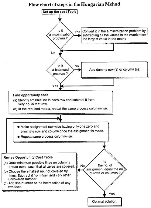
The Hungarian method are often summarized within the following steps.
Step 1: Create a price table from the given problem.
If the amount of rows isn't adequate to the amount of columns, or the other way around, you would like to feature dummy rows or columns. The value of allocating dummy cells is usually zero.
Step 2: Find the chance Cost Table:
(A) Find the littlest element in each row of the required cost table and subtract it from each element therein row.
(B) Within the reduction matrix obtained from 2 (a), find the littlest element in each column and subtract it from each element. Each row and column has a minimum of one zero value.
Step 3: Make an allocation within the cost Matrix:
The allocation procedure is as follows:
(A) Examine the rows continuously until you get a row with just one unmarked zero. Make the assignment one zero by creating a square around it.
(B) For every zero value assigned, delete (cancel) all other zeros within the same row and / or column.
(C) Repeat steps 3 (a) and three (b) for every column, leaving just one unassigned zero value.
(D) If there are two or more unmarked zeros within the rows and / or columns and therefore the check cannot select one, select any assigned zero cell.
(E) Continue this process until all zeros within the matrix are enclosed (assigned) or deleted (x).
Step 4: Optimal criteria:
If the assigned cell members are adequate to the row sequence that is the best solution. The entire cost related to this solution is obtained by adding the first cost figure to the occupied cell.
If zero cells are arbitrarily selected in step (3), an alternate optimal solution exists. However, if you can't find the simplest solution, attend step (5).
Step 5: Modify the chance cost table.
Use the subsequent procedure to draw a group of horizontal and vertical lines that cover all zeros within the revised cost table obtained in step (3).
(A) Add a check (√) to every row that has not been assigned.
(B) Examine the marked line. If zeros occur in these columns, check each row that contains the assigned zeros.
(C) Repeat this process until you'll not mark rows or columns.
(D) Draw a line through each marked column and every unmarked row.
If the amount of drawn lines is adequate to the amount (or columns), then the present solution is that the best solution otherwise, attend step 6.
Step 6: Create a newly revised cost Table.
(A) Select the littlest element from the cells that aren't covered by the road, and call this value K.
(B) Draw K from all the weather within the cell that isn’t covered by the road.
(C) Add K to the element within the cell covered by the 2 lines, that is, the intersection of the 2 lines.
(D) The weather of the cell covered by one row aren't changed.
Step 7: Repeat steps 3-6 close up the lights for the simplest solution
Case study
Example: At the Computer Center, after careful study of the three expert programs responsible for the Computer Center, the experts estimate the computer time required for the application program in minutes as follows:
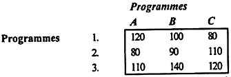
Assign programmers to the program to minimize the total computer time.
Solution:
Hungarian law is used to obtain the optimal solution.
Steps (1) & (2):
The minimum time elements for lines 1, 2, and 3 are 80, 80, and 110. Subtract these elements from all the elements in each row.
The shortened time matrix is shown in Table (1) below table 1:
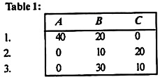
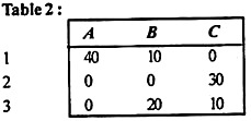
In the reduced table (1), the minimum time elements in columns A, B, and C are 0, 10, and 0, and these elements are subtracted from all of these elements columns for getting the shortened time matrix, as shown in Table 2.
Step 3 (a):
Examine all rows, starting with the first row and until you find a row that contains only a single zero element. Here, rows 1 and 3 have only one zero in each of cells (1, C) and (3, A) assigned these zeros. All zeros in the assigned column are erased, as shown in Table 3.
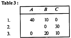
(B) Now look at each column starting with A in Table 3. There is one zero in column B of cell (2, B). Allocate this cell as shown in Table 4.
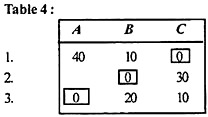
(C) The number of allocations (= 3) is equal to the number of rows (= 3), so the optimal solution is obtained. The pattern of allocation between the programmer and the program and each line (in minutes) is shown below.

Example 2:
The department has five employees and needs to perform five tasks. The time it takes for each man to perform each task (in hours) is shown in the effectiveness matrix.
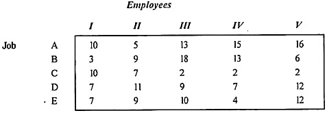
How do I need to assign one job to each employee to minimize total man-hours?
Solution:
Applying step (1) and step (2) of the algorithm (2) gives an opportunity reduction time matrix as shown in Table (1).

In the reduced table (1), the minimum time elements in columns I, II, III, IV, and V are 0, 0, 0, 0, 0, respectively, and we subtract these from each element. The columns get the same reduced matrix.
Step 3 (a):
Examine all rows one at a time, starting with A and until you find a row that contains only a single zero element H.. All zeros in the assigned column are deleted, as shown in Table 2.
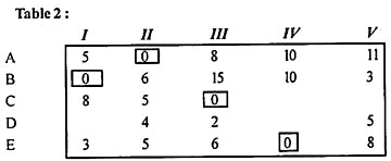
(B) Now, start with the columns and examine each column. 1. There is one zero in column III. Cell (C, III) Allocation is made in this cell. Therefore, cells (C, V) are crossed off. As shown in Table 2, all zeros in the table are assigned or cleared.
The solution is not optimal as only four assignments are made.
Step 4:
Cover zeros with the minimum number of rows (= 4), as described below.
(A) Line D has no assignment, so mark line (√) line D.
(B) Mark (√) columns I and IV because row D has zero elements in these columns.
(C) Mark (√) rows B and E because (c) columns 1 and (IV) have assignments for rows B and E, respectively.
(D) Draw a straight line through unmarked rows A and C and marked columns I and IV, as other rows or columns cannot be marked, as shown in Table 3.
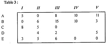
Step 5:
Create a new revised table by selecting the smallest element from all the uncovered elements in the rows of Table 3. , 1), (A, IV), (C, 1) <and (E, IV) respectively. It is at the intersection of the two lines. Table 4 shows another revised table thus obtained.
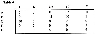
Step 7:
Repeat steps (3) through (5) to find a new solution. The new assignments are shown in Table 5.
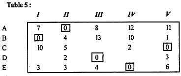
The solution is best if the number of allocations (= 5) is equal to the number of rows (or columns).
The patterns of allocation between jobs and employees and their respective hours (in hours) are shown below.

Variations on the assignment problem:
Disproportionate allocation problem:
If the cost matrix is not a square matrix, that is, the number of rows and columns are not equal, the allocation problem is said to be imbalanced. Add a dummy row or column with all entries zero for balance.
Example 3:
There are four jobs assigned to the machine. In the following matrix, you can assign only one job to a machine.

Find the best job assignments for machines, minimize total processing time, and also find out which machines have no jobs assigned. What is the total processing time to complete all jobs?
Solution:
The problem is imbalanced because the cost matrix is not a square matrix. Add dummy job 5 with zero corresponding entry modified matrix.
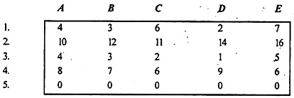
Steps 1 & 2:
Subtract the smallest element from all the elements in each row and column.

Steps 3 & 4:
Now, do the zero allocation in the usual way and get the next matrix.

However, the solution is not optimal because there are only four allocations.
Step 5:
In this step, draw the minimum number of the line that covers zeros.

Rows covering all zeros = 4 <matrix order. The minimum uncovered element (i) is subtracted from the remaining uncovered elements and added to the element at the intersection of the lines to form the second modified matrix.
Step 6:
Repeat steps (3) and (4) again to find the next matrix.
Here, the total number of allocations (= 5) is equal to the number of rows or columns. Then this is the best solution.
The allocation pattern is shown below.

For machine E, no jobs have been assigned. Optimal (minimum)
Cost = 10 + 3 + 6 + 1 = Rs.20
Case study- Airline crew assignment
Example 4: (Airline crew assignment)
Below is a timetable for airlines that operate seven days a week. Crew members must have a flight interval of at least 6 hours. Get a pair of flights that minimizes transit time from home. With any pairing, the crew is based in one city, resulting in fewer connections.
Solution:
If your crew is based in Delhi, first create a table of possible connections between flights. The time difference between Flight I and Flight 101 is 24 hours. That is 1,440 minutes, but the minimum transfer required is 6 hours or 360 minutes.
If the crew is based in Delhi, the layover table would look like this:

Similarly, create a transit table for Calcutta-based crew members.

According to the given constraints, the minimum layover times are shown in the following table.

The circled numbers indicate the connections of the Calcutta-based crew, while the encircled numbers indicate the Delhi-based crew.
Step 1:
Subtracting the minimum element of each row from all the elements of the corresponding row gives:

Step 2:
Subtract the column that is minimum from all elements of the column.

Step 3:
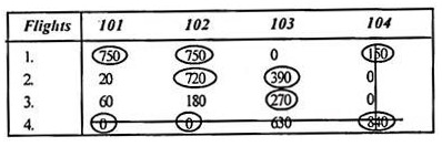
Since optimal allocation is not possible in a given situation, assigning to a zero element draws a minimum number of horizontal or vertical lines to cover all zeros, and three as shown below. Get the line.

This number is not equal to the number of rows / columns, so 3 rows are retrieved. The solution is not optimal. Proceed to step (4).
Step 4:
Identify the smallest uncovered element and subtract it from all uncovered elements. In addition to the intersection elements, the matrix is modified as follows (minimum element = 60).
Step 5:
(Repeat step 3) Draw a horizontal vertical line to cover all zeros:

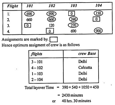
The number of rows is now equal to the row sequence (that is, 4). Therefore, the solution is optimal. Proceed to step (6).
Step 6:
Assign to zero element
Maximum 5 x 5 Matrix. Up to Maximum Two Iterations after Row and Column Minimization:
Example: Five salesmen are to be assigned to five districts. Estimates of sales revenue (in thousands) for each salesman are given as follows-
| A | B | C | D | E |
1 | 32 | 38 | 40 | 28 | 40 |
2 | 40 | 24 | 28 | 21 | 36 |
3 | 41 | 27 | 33 | 30 | 37 |
4 | 22 | 38 | 41 | 36 | 36 |
5 | 29 | 33 | 40 | 35 | 39 |
Find the assignment pattern that maximises the sales revenue.
Sol.
In order to maximize the sales revenue we have to convert this into minimisation form before proceeding to the Hungarian method.
For this, we obtain the opportunity loss matrix by subtracting every element in the given table from the largest element in it. In this case, the largest element is 41.
Thus, we obtain the following opportunity loss matrix:
9 | 3 | 1 | 13 | 1 |
1 | 17 | 13 | 20 | 5 |
0 | 14 | 8 | 11 | 4 |
19 | 3 | 0 | 5 | 5 |
12 | 8 | 1 | 6 | 2 |
Now we apply Hungarian method, we get-

Since the number of assigned zeroes is less than the number of rows, we apply next step of the Hungarian method and draw the minimum number of horizontal/vertical lines that cover all the zeroes as shown in the following
Table-
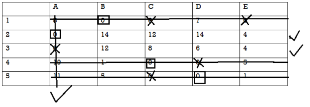
Select the minimum element from amongst the uncovered elements, which is 4 in this case. We subtract the element 4 from each of the uncovered elements and add it to the elements which lie at the intersection of the horizontal and vertical lines. Other covered elements remain unaltered.
Then applying the Hungarian method to the resulting matrix, we get

Since the number of assigned zeroes is equal to the number of rows, the optimum assignment has been attained and is given as:
1  B, 2
B, 2 A, 3
A, 3 E, 4
E, 4 C, 5
C, 5 D
D
So that, the maximum sales revenue = 38 + 40 + 37 + 41 + 35 thousand rupees
= 191 thousand rupees.
Key takeaways:
1. Hungarian method of solving assignment problems is based on two important properties:
2. In given cost matrix, if a constant quantity is added or subtracted from every element of any row or column, an assignment that minimizes the total cost in one matrix also minimizes the total cost in the other.
3. For an assignment problem having all non-negative cost, a solution having zero total cost is an optimum solution.
4. Assignment Problem may not necessarily have an optimal solution. It may also have multiple solutions to a given problem.
References:
- Operations research- theory and application, JK Sharma, trinity press
- Operations research, P. Rama Murthy, new age international publishers
- Higher engineering mathematics, B.S. Gerewal
- Operations research by kanti swarup
