Unit - 1

Probability

1.1 Probability: Introduction, Sample spaces, Events, probability of events, rules of probability

Probability is the study of chances. Probability is the measurement of the degree of uncertainty and therefore, of certainty of the occurrence of events.

A probability space is a three-tuple (S, F, P) in which the three components are

1. Sample space: A nonempty set S called the sample space, which represents           all possible outcomes.
2. Event space: A collection F of subsets of S, called the event space.
3. Probability function: A function P : FR, that assigns probabilities to the events in F.

DEFINITIONS:

1. Die: It is a small cube. Dots (number) are marked on its faces. Plural of the die is dice. On throwing a die, the outcome is the number of dots on its upper face.

2. Cards: A pack of cards consists of four suits i.e. Spades, Hearts, Diamonds and Clubs. Each suit consists of 13 cards, nine cards numbered 2, 3, 4, ..., 10, an Ace, a King, a Queen and a Jack or Knave. Colour of Spades and Clubs is black and that of Hearts and Diamonds is red.

Kings, Queens and Jacks are known as face cards.

3. Exhaustive Events or Sample Space: The set of all possible outcomes of a single performance of an experiment is exhaustive events or sample space. Each outcome is called a sample point.

In case of tossing a coin once, S = (H, T) is the sample space. Two outcomes - Head and Tail

- constitute an exhaustive event because no other outcome is possible.

4. Random Experiment: There are experiments, in which results may be altogether different, even though they are performed under identical conditions. They are known as random experiments. Tossing a coin or throwing a die is random experiment.

5. Trial and Event: Performing a random experiment is called a trial and outcome is termed as event. Tossing of a coin is a trial and the turning up of head or tail is an event.

6. Equally likely events: Two events are said to be ‘equally likely’, if one of them cannot be expected in preference to the other. For instance, if we draw a card from well-shuffled pack, we may get any card. Then the 52 different cases are equally likely.

7. Independent events: Two events may be independent, when the actual happening of one does not influence in any way the probability of the happening of the other.

8. Mutually Exclusive events: Two events are known as mutually exclusive, when the occurrence of one of them excludes the occurrence of the other. For example, on tossing of a coin, either we get head or tail, but not both.

9. Compound Event: When two or more events occur in composition with each other, the simultaneous occurrence is called a compound event. When a die is thrown, getting a 5 or 6 is a compound event.

10. Favourable Events: The events, which ensure the required happening, are said to be favourable events. For example, in throwing a die, to have the even numbers, 2, 4 and 6 are favourable cases.

11. Conditional Probability: The probability of happening an event A, such that event B has already happened, is called the conditional probability of happening of A on the condition that B has already happened. It is usually denoted by

12. Odds in favour of an event and odds against an event: If number of favourable ways = m, number of not favourable events = n

(i) Odds in favour of the event

(ii) Odds against the event

Classical definition of probability-

Suppose there are ‘n’ exhaustive cases in a random experiment which is equally likely and mutually exclusive.

Let ‘m’ cases are favourable for the happening of an event A, then the probability of happening event A can be defined as-

Probability of non-happening of the event A is defined as-

Note- Always remember that the probability of any events lies between 0 and 1.

Expected value-

Let are the probabilities of events and respectively. Then the expected value can be defined as-

Example: A bag contains 7 red and 8 black balls then find the probability of getting a red ball.

Sol.

Here total cases = 7 + 8 = 15

According to the definition of probability,

So that, here favourable cases-  red balls = 7

Then,

Addition and multiplication law of probability-

Addition law-

If are the probabilities of mutually exclusive events, then the probability P, that any of these events will happen is given by

Note-

If two events A and B are not mutually exclusive then then probability of the event that either A or B or both will happen is given by-

Example: A box contains 4 white and 2 black balls and a second box contains three balls of each colour. Now a bag is selected at random and a ball is drawn randomly from the chosen box. Then what will be the probability that the ball is white.

Sol.

Here we have two mutually exclusive cases-

1. The first bag is chosen

2. The second bag is chosen

The chance of choosing the first bag is 1/2. And if this bag is chosen then the probability of drawing a white ball is 4/6.

So that the probability of drawing a white ball from first bag is-

And the probability of drawing a white ball from second bag is-

Here the events are mutually exclusive, then the required probability is-
 

Example-25 lottery tickets are marked with first 25 numerals. A ticket is drawn at random.

Find the probability that it is a multiple of 5 or 7.

Sol:

Let A be the event that the drawn ticket bears a number multiple of 5 and B be the event that it bears a number multiple of 7.

So that

A = {5, 10, 15, 20, 25}

B = {7, 14, 21}

Here, as A B = ,

A and B are mutually exclusive

Then,

Multiplication law-

For two events A and B-

Here is called conditional probability of B given that A has already happened.

Now-

If A and B are two independent events, then-

Because in case of independent events- 

Example: A bag contains 9 balls, two of which are red three blue and four black.

Three balls are drawn randomly. What is the probability that-

1. The three balls are of different colours

2. The three balls are of the same colours.

Sol.

1. Three balls will be of different colour if one ball is red, one blue and one black ball are drawn-

Then the probability will be-

2. Three balls will be of same colour if one ball is red, one blue and one black ball are drawn-

Then the probability will be-

Example: A die is rolled. If the outcome is a number greater than three. What is the probability that it is a prime number.

Sol.

The sample space is-   S = {1, 2, 3, 4, 5, 6}

Let A be the event that the outcome is a number which is greater than three and  B be the event that it is a prime.

So that-

A = {4, 5, 6} and B = {2, 3, 5} and hence

P(A) = 3/6, P(B) = 3/6 and

Now the required probability-

Example: Two cards are drawn from a pack of playing cards in succession with replacement of first card. Find the probability that the both are the cards of heart.

Sol.

Let A be the event that first card drawn is a heart and B be the event that second card is a heart card.

As the cards are drawn with replacement,

Here A and B are independent and the required probability will be-

Example: Two male and female candidates appear in an interview for two positions in the same post. The probability that the male candidate is selected is 1/7 and the female candidate selected is 1/5.

What is the probability that-

1. Both of them will be selected

2. Only one of them will be selected

3. None of them will be selected.

Sol.

Here, P (male’s selection) = 1/7

And

P (female’s selection) = 1/5

Then-

1.

2.

3.

Example: A can hit a target 3 times in 5 shots, B 2 times in 5 shots and C 3 times in 4 shots. All of them fire one shot each simultaneously at the target.

What is the probability that-

1. Two shots hit

2. At least two shots hit

Sol.

1. Now probability that 2 shots hit the target-

2.

Probability of at least two shots hitting the target

Key takeaways-

1. Exhaustive Events or Sample Space: The set of all possible outcomes of a single performance of an experiment is exhaustive events or sample space. Each outcome is called a sample point.
2. Equally likely events: Two events are said to be ‘equally likely’, if one of them cannot be expected in preference to the other.
3. Independent events: Two events may be independent, when the actual happening of one does not influence in any way the probability of the happening of the other.
4. Mutually Exclusive events: Two events are known as mutually exclusive, when the occurrence of one of them excludes the occurrence of the other.
5. Conditional Probability: The probability of happening an event A, such that event B has already happened, is called the conditional probability of happening of A on the condition that B has already happened. It is usually denoted by
6. Classical Definition of Probability. If there are N equally likely, mutually, exclusive and exhaustive of events of an experiment and m of these are favourable, then the probability of the happening of the event is defined as

1.2 Conditional probability, Independent events

Let A and B be two events of a sample space Sand let . Then conditional probability of the event A, given B, denoted byis defined by –

Theorem: If the events A and B defined on a sample space S of a random experiment are independent, then

Example1: A factory has two machines A and B making 60% and 40% respectively of the total production. Machine A produces 3% defective items, and B produces 5% defective items. Find the probability that a given defective part came from A.

SOLUTION:

We consider the following events:

A: Selected item comes from A.

B: Selected item comes from B.

D: Selected item is defective.

We are looking for . We know:

Now,

So we need

Since, D is the union of the mutually exclusive events and (the entire sample space is the union of the mutually exclusive events A and B)

Example2: Two fair dice are rolled, 1 red and 1 blue. The Sample Space is

S = {(1, 1),(1, 2), . . . ,(1, 6), . . . ,(6, 6)}.Total -36 outcomes, all equally likely (here (2, 3) denotes the outcome where the red die show 2 and the blue one shows 3).

(a) Consider the following events:

A: Red die shows 6.

B: Blue die shows 6.

Find, and .

Solution:

NOTE:

so for this example. This is not surprising - we expect A to occur in of cases. In of these cases i.e. in of all cases, we expect B to also occur.

(b) Consider the following events:

C: Total Score is 10.

D: Red die shows an even number.

Find , and .

Solution:

NOTE:

so,.

Why does multiplication not apply here as in part (a)?

ANSWER: Suppose C occurs: so the outcome is either (4, 6), (5, 5) or (6, 4). In two of these cases, namely (4, 6) and (6, 4), the event D also occurs. Thus

Although , the probability that D occurs given that C occurs is .

We write, and call the conditional probability of D given C.

NOTE: In the above example

Example3: Three urns contain 6 red, 4 black; 4 red, 6 black; 5 red, 5 black balls respectively. One of the urns is selected at random and a ball is drawn from it. If the ball drawn is red find the probability that it is drawn from the first urn.

Solution:

: The ball is drawn from urn I.

: The ball is drawn from urn II.

: The ball is drawn from urn III.

R: The ball is red.

We have to find

Since the three urns are equally likely to be selected

Also,

From (i), we have

Example: A bag contains 12 pens of which 4 are defective. Three pens are picked at random from the bag one after the other.

Then find the probability that all three are non-defective.

Sol. Here the probability of the first which will be non-defective = 8/12

By the multiplication theorem of probability,

If we draw pens one after the other then the required probability will be-

Example: The probability of A hits the target is 1 / 4 and the probability that B hits the target is 2/ 5. If both shoot the target then find the probability that at least one of them hits the target.

Sol.

Here it is given that-

Now we have to find-

Both two events are independent. So that-

Independence:

Two events A, B ∈ are statistically independent iff

(Two disjoint events are not independent.)

Independence implies that

Knowing that outcome is in B does not change your perception of the outcome’s being in A.

Key takeaways-

1.4 Bayes’s theorem

If , are mutually exclusive events with of a random experiment then for any arbitrary event of the sample space of the above experiment with , we have

(for )

Example1: An urn contains 3 white and 4 red balls and an urn lI contains 5 white and 6 red balls. One ball is drawn at random from one ofthe urns and isfound to be white. Find the probability that it was drawn from urn 1.

Solution: Let : the ball is drawn from urn I

: the ball is drawn from urn II

: the ball is white.

We have to find

By Bayes Theorem

... (1)

Since two urns are equally likely to be selected, (a white ball is drawn from urn )

(a white ball is drawn from urn II)

From(1),

Example2: Three urns contains 6 red, 4 black, 4 red, 6 black; 5 red, 5 black balls respectively. One of the urns is selected at random and a ball is drawn from it. Lf the ball drawn is red find the probability that it is drawn from thefirst urn.

Solution:

Let : the ball is drawn from urn 1.

: the ball is drawn from urn lI.

: the ball is drawn from urn 111.

: the ball is red.

We have to find .

By Baye’s Theorem,

... (1)

Since the three urns are equally likely to be selected

Also (a red ball is drawn from urn )

(R/) (a red ball is drawn from urn II)

(a red ball is drawn from urn III)

From (1), we have

Example3: ln a bolt factory machines and manufacturerespectively 25%, 35% and 40% of the total. Lf their output 5, 4 and 2 per cent are defective bolts. A bolt is drawn at random from the product and is found to be defective. What is the probability that it was manufactured by machine B.?

Solution: bolt is manufactured by machine

: bolt is manufactured by machine

: bolt is manufactured by machine

The probability ofdrawing a defective bolt manufactured by machine is (D/A)

Similarly, (D/B) and (D/C)

By Baye’s theorem

Key takeaways:

1.3 Probability distributions and probability densities: random variables, probability distributions continuous random variables, probability density functions

Random Variable:

It is a real valued function which assign a real number to each sample point in the sample space.

A random variable is said to be discrete if it has either a finite or a countable number of values

The number of students present each day in a class during an academic session is an example of discrete random variable as the number cannot take a fractional value.

A random variable X is a function defined on the sample space 5 of an experiment S of an experiment. Its value are real numbers. For every number a the probability

With which X assumes a is defined. Similarly for any interval l the probability

With which X assumes any value in I is defined.

Example: 1. Tossing a fair coin thrice then-

Sample Space(S) = {HHH, HHT, HTH, THH, HTT, THT, TTH, TTT}

2. Roll a dice

Sample Space(S) = {1,2,3,4,5,6}

Probability mass function-

Let X be a r.v. Which takes the values and let P[X = ] = p(. This function p(xi), i =1,2, … defined for the values assumed by X is called probability mass function of X satisfying p(xi) ≥0 and

Example: A random variable x has the following probability distribution-

Then find-

1. Value of c.

2. P[X≤3]

3. P[1 < X <4]

Sol.

We know that for the given probability distribution-

So that-

2.

3.

Discrete Random Variable:

A random variable which takes finite or as most countable number of values is called discrete random variable.

Discrete Random Variables and Distribution

By definition a random variable X and its distribution are discrete if X assumes only finitely maany or at most contably many values called the possible values of X. With positive probabilities is zero for any interval J containing no possible values.

Clearly the discrete distribution of X is also determined by the probability functions f (x) of X, defined by

From this we get the values of the distribution function F (x) by taking sums.

Discrete Probability Distributions

Each event in a sample space has certain probability (or chance) of occurrence (or happening). A formula representing all these probabilities which a discrete random variable assumes, is known as the discrete probability distribution.

Discrete probability distribution, probability function or probability mass function of a discrete random variable X is the function f (x) satisfying the following conditions:

Thus probability distribution is the set of ordered pairs (x, f (x)), i.e., outcome x and its probability (chance) f (x). Cumulative distribution or simply distribution of a discrete random variable X is F (x) defined by

It follows that,

Continuous Random Variables

A random variable X is said to be continuous R.V. If S contains infinite numbers equal to the number of points on a line segment.

Continuous Probability Distributions

For a continuous R.V. X, the function f (x) satisfying the following, is known as the probability density function (P.D.F.) or simply density function

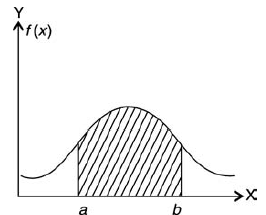
area under f (x) between ordinates x = a and x = b.

Note- P (a < X < b) = P (a ≤ X < b) = P (a < X ≤ b) = P (a ≤ X ≤ b)

Probability density function-

Suppose f( x ) be a continuous function of x . Suppose the shaded region ABCDshown in the following figure represents the area bounded by y = f( x ), x –axis and the ordinates at the points x and x + δx , where δxis the length of the interval ( x , x + δx ).ifδx is very-very small, then the curve AB will act as a line and hence the shaded region will be a rectangle whose area will be AD × DCthis area = probability that X lies in the interval ( x, x +δx )

= P[ x≤ X ≤ x +δx ]

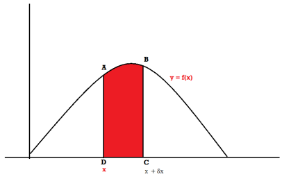
Hence,

Example: If a continuous random variable X has the following probability density function:

Then find-

1. P[0.2 < X < 0.5]

Sol.

Here f(x) is the probability density function, then-

Distribution functions and densities

A function F defined for all values of a random variable X by

F( x ) = P[X ≤ x ] is called the distribution function. It is also known as the cumulative distribution function (c.d.f.) of X since it is the cumulative probability of X up to and including the value x.

Continuous Distribution Function

Distribution function of a continuous random variable is called the continuous distribution function or cumulative distribution function (c.d.f.).

Let X be a continuous random variable having the probability density function

f( x ), as defined in the last section of this unit, then the distribution function

F( x ) is given by

Example: The pdf of a continuous random variable is given as below-

Then find the c.d.f. Of X.

Sol.

The c.d.f. Of X will be given by-

Hence the c.d.f will be-

Independent random variables

Two discrete random variables X and Y are said to be independent only if-

Note- Two events are independent only if

Example: Two discrete random variables X and Y have-

And

P[X = 1, Y = 1] = 5/9.

Check whether X and Y are independent or not?

Sol.

First we write the given distribution In tabular form-

Now-

But

So that-

Hence X and Y are not independent.

Key takeaways-

1. Two discrete random variables X and Y are said to be independent only if-

2.      Two events are independent only if

3.      Two events A, B ∈ are statistically independent iff

4.     Independence implies that

3.

1.4 Multivariate distributions, joint distribution function

Bivariate discrete random variables-

Let X and Y be two discrete random variables defined on the sample space S of a random experiment then the function (X, Y) defined on the same sample space is called a two-dimensional discrete random variable. In other words, (X, Y) is a two-dimensional random variable if the possible values of (X, Y) are finite or countably infinite. Here, each value of X and Y is represented as a point ( x, y ) in the xy-plane.

Joint probability mass function-

Let (X, Y) be two-dimensional discrete random variables with each possible outcome , we associate a number representing-

And satisfying the given conditions-

The function p defined for all is called joint probability mass function of X and Y.

Conditional probability mass function-

Let (X, Y) be a discrete two-dimensional random variable. Then the conditional probability mass function of X, given Y = y is defined as-

Because-

A bivariate distribution, setonly, is the probability that a definite event will happen when there are 2 independent random variables in your scenario. E.g, having two bowls, individually complete with 2dissimilarkinds of candies, and drawing one candy from each bowl gives you 2 independent random variables, the 2dissimilar candies. Since you are pulling one candy from each bowl at the same time, you have a bivariate distribution when calculating your probability of finish up with specific types of candies.

Properties:

Property 1

Two random variable X and V are said to be bivariate normal, or jointly normal, if aX +bY has a normal distribution for all a,

Properties 2:

Two random variable X and V are said to be standard bivariate normal distribution with correlation coefficient if their joint PDF is given by

Where . If , then we just say X and Y have the standard bivirate normal distribution.

Properties 3:

Two random variable X and V are said to be bivariate normal distribution with parameters if their joint PDF is given by

Where, and are all constants

Properties 4:

Suppose X and Y are jointly variables with parameters . Then given X=x,Y is normally distributed with

Example 1:

Let be two independent N(0,1) random variables. Define

Where is a real number in (-1,1)

a. Show that X and Y are bivariate normal.

b. Find the joint PDF of X and Y.

c. Find (X,Y)

Sol. First, note that since are normal and independent , they are jointly normal with the joint PDF

We need to show aX+bY is normal for all we have

and thus it is normal.

We can use the methods of transformations (Theorem 5.1) to find the joint PDF of X and Y . The inverse transformation is given by

Thus we conclude that,

To find , first mode

Therefore,

Example 2:

Let X and Y be jointly normal random variables with parameters Find the conditional distribution of Y given X =x.

Sol. One way to solve this problem is by using the joint PDF formula since X N we can use

Thus given X=x, we have

And,

Since are independent, knowing does not provide any information on . We have shown that given X=x,Y is a linear function of , thus it is normal. Ln particular

We conclude that given X=x,Y is normally distributed with mean and variance
 

Example 3;

Let X and Y be jointly normal random variables with parameters
 

Find

Find

Find

Sol. a. Since X and Y are jointly normal, the random variable V-2X+Y is normal. We have

Thus, , therefore,

Note that

Using Properties, we conclude that given X=2,Y is normally distributed with

Thus,

1.5 Joint probability density function, marginal distributions

Joint probability distribution:

Let S be a sample space associated with a random experiment ε. Let X = X(s) and Y = Y (s) be two random variables on the same sample space S. The two real valued functions X(s) and Y (s) each assign a real number to each outcome s of the sample space S, with respective image sets given by X(s) = {X(s1), X(s2 ), . . . , X(sn)}={X1, X2 , . . . , Xn} and Y (s) = {Y (s1), Y (s2 ), . . . , Y (sm)}={Y1, Y2 , . . . , Ym}

Here the two random variables X and Y are discrete since the possible values of X and Y are finite (or countably infinite).

Example:

a. X: Age, Y : Blood pressure of a person.

b. X: Crop yield, Y : Rain fall in an area.

c. X: I.Q., Y : Nutrition of an individual.

Consider the product set

X(S) × Y (S) = {(x1, y1), (x1, y2 ), . . . , (xn, ym)} .

The joint probability distribution or joint distribution or probability mass function or joint probability function of two discrete random variables

X and Y is a function h(x, y) difined on the product set X(s) × Y (s) assigning probability to each of the ordered pairs (xi , yi ).

Thus h(xi , yi ) = P(X = xi , Y = yj ) gives the probability for the simultaneous occurrences of the outcomes xi and yi . Further h(x, y) satisfies the following:

The set of triplets (xi , yj , h(xi , yj )) for i = 1 to n, j = 1 to m, known as the probability distribution of the two random variables X, Y is in general represented in the form of a rectangular table as follows:

Marginal Distributions

Marginal distribution f (x) of X is the probability distribution of X alone; obtained by summing h(x, y) over the values of Y . i.e.,

Or f (xi ) is the row sum of the ith row entries. Similarly, marginal distribution g(y) of Y is the probability distribution of Y alone, obtained by summing h(x, y) over the values of X. i.e.,

Or g(yj ) is the column sum of the j th column entries.

Example: Find the joint distribution of X and Y , which are independent random variables with the following respective distributions:

Since X and Y are independent random variables, h (xi , yj ) = f (xi ) g(yj ). Thus the entries of the joint distribution are the products of the marginal entries

Example: Two cards are selected at a random from a box which contains five cards numbered 1, 1, 2, 2 and 3. Find the joint distribution of X and Y where X denotes the sum and Y, the maximum of the two numbers drawn.

Sol:

The possible pair of numbers are (1,1),

(1,1), (1,2), (2,1), (1,2), (2,1), (1,3), (3,1), (2,2), (2,3), (3,2). Sum of two numbers are 2, 3, 4, 5 while maximum numbers are 1, 2, 3. Thus

Distribution of X is

Distribution of Y is

Joint distribution is

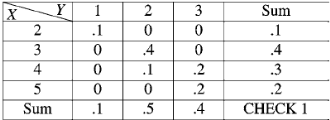
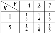
Example: Find (a) marginal distributions f (x) and g(y)

Sol:

The marginal distribution f (x) is obtained by row sums and g(y) by column sums.

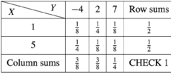
The marginal distribution f (x):

The marginal distribution g(y):

Example: Find the joint distribution of X and

Y , which are independent random variables with the

Following respective distributions:

	1	2
P [ X =	0.7	0.3

And

	-2	5	8
P [ Y =	0.3	0.5	0.2

Sol.

Since X and Y are independent random variables,

Thus the entries of the joint distribution are the products of the marginal entries

Example: The following table represents the joint probability distribution of

The discrete random variable (X, Y):

Then find-

i) The marginal distributions.

Ii) The conditional distribution of X given Y = 1.

Iii) P[(X + Y) < 4].

Sol.

i) The marginal distributions.

The marginal probability distribution of X is-

The marginal probability distribution of Y is

Ii) The conditional distribution of X given Y = 1.

The conditional distribution of X given Y = 1 is-

X	1	2	3
	¼	1/4	½

(iii) The values of (X, Y) which satisfy X + Y < 4 are (1, 1), (1, 2) and (2, 1)

Only.

Which gives-

Example: Find-

(a) Marginal distributions

(b) E(X) and E(Y )

(c) Cov (X, Y )

(d) σX , σY and

(e)  ρ(X, Y )

For the following joint probability distribution-

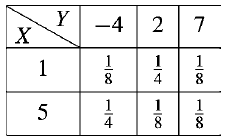
Sol.

(a) Marginal distributions

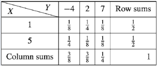
The marginal distribution of x

The marginal distribution of Y-

(b) E(X) and E(Y )

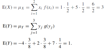
(c) Cov (X, Y )

As we know that-

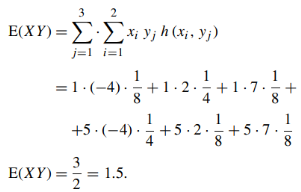
= -1.5

(d) σX , σY and

(e)  ρ(X, Y )

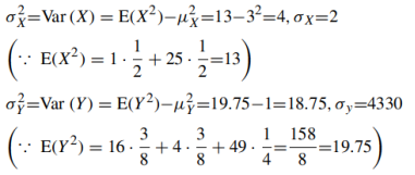
1.6 Conditional distributions, conditional density

Conditional Probability Distributions

Conditional distribution of random variable Y given that X = x is

Similarly, the conditional distribution of X given that Y = y is

Thus

Where the summation is for all values of X between a and b.

In probability theory assumed two jointly distributed R.V. X & Y{\displaystyle X}{\displaystyle Y} the conditional probability distribution of Y given X is the probability distribution of Y {\displaystyle Y}when X {\displaystyle X}is known to be a precise value; in some suitcases the conditional probabilities may be stated as functions containing the unnamed value {\displaystyle x}XXof X {\displaystyle X}XX  as a limitation. Once together X {\displaystyle X}xand Y{\displaystyle Y}are given variables, a conditional probability is characteristically used to indicate the conditional probability. The conditional distribution differences with the marginal distribution of a random variable, which is distribution deprived of reference to the value of the additional variable.

If conditional distribution of Y {\displaystyle Y}under X{\displaystyle X} is a continuous distribution, then probability density function is called as conditional density function. The properties of a conditional distribution, such as the moments, are frequently denoted to by corresponding names such as the conditional mean and conditional variance.

Let A and B be two events of a sample space S and let . Then conditional probability of the event A, given B, denoted by P (A/B) is defined by

Theorem. If the events A and B defined on a sample space S of a random experiment are independent then

Proof. A and B are given to be independent events.

Example: A die is tossed. If the number is odd, what is the probability that it is prime?

Sol:

2, 4, 6, are even, 1, 3, 5 are three odd numbers, of which two are prime numbers (namely

3 and 5) Conditional probability is w.r.t. the reduced sample space of odd numbers only. Thus

P (Prime given odd) = P (P /O) = 2/3

Example: Two digits are selected at random from the digits 1 through 9 (a) If the sum is odd, what is the probability that 2 is one of the numbers selected (b) If 2 is one of the digits selected, what is the probability that the sum is odd?

Sol:

We know that even + even = even, odd + odd = even and odd + even = odd.

a. Odd = {1, 3, 5, 7, 9}, even = {2, 4, 6, 8}

Since the sum is odd it must be the sum of an odd number and an even number i.e., odd= odd+ even

P (2 selected) = ¼

b. 2 is selected, so the other number must be odd number

P (sum is odd/2 is selected) = 5/8

Example: A box contains 9 tickets numbered 1 to 9 inclusive. If 3 tickets are drawn from the box one at a time, find the probability they are alternatively either odd, even, odd or even, odd, even.

Sol: 4 even numbers = {2, 4, 6, 8},

5 odd numbers = {1, 3, 5, 7, 9}.

Let e denote even and o denote odd number

P (oeo or eoe) = P (oeo) + P (eoe)

Since oeo and eoe are mutually exclusive. Now

Prob(odd and even and odd) = P (odd) P (even/given

Odd) P (odd/given odd and even)

P (oeo) = P (o)P (e/o)P (o/oe) = 5/9. 4/8 . 4/7 = 10/63

Similarly,

P (eoe) = P (e)P (o/e)P (e/eo)

P (eoe) = 4/9 . 5/8 . 3/7 = 5/42

So P (oeo or eoe) = 10/63 + 5/ 42 = 5/18

Key takeaways:

1. 
2. 
3. If the events A and B defined on a sample space S of a random experiment are independent then

1.7 The theory in practice, data analysis, frequency distribution, class limits, class frequencies, class boundary, class interval, class mark, skewed data, multimodality, graphical representation of the data, measures of location and variability

Classification of data:

Classification of data is a function very similar to that of sorting letters in a post office. Let us explain it further by considering a situation where university receives applications of candidates for filling up some posts for its various departments or disciplines. The applications received for the posts in the university are sorted according to the departments or disciplines to which they pertain. It is well known that the applications collected in an office are sorted into different lots, department or discipline wise, i.e. in accordance with their destinations as Social Sciences, Engineering, Basic Sciences, etc. They are then put in separate belongings each containing applications with a common characteristic, viz, having the same discipline. Classification of statistical data is comparable to the categorisation process. The process of classification gives distinction to important information gathered, while dropping unnecessary facts, enables comparison and a statistical treatment of the material collected.

Types of Classification

Broadly, data can be classified under following categories:

(i) Geographical classification

(ii) Chronological classification

(iii) Qualitative classification

(iv) Quantitative classification

Let us discuss these one by one:

(i) Geographical Classification

In geographical classification, data are classified on the basis of location, region, etc.

(ii) Chronological Classification

Classification of data observed over a period of time is known as chronological classification.

(iii) Quantitative Classification

Quantitative classification refers to the classification of data according to some characteristics that can be measured numerically such as height, weight, income, age, sales, etc.

(iv) Qualitative Classification

In qualitative classification, data are classified on the basis of some attributes or qualitative characteristics such as sex, colour of hair, literacy, religion, etc.

Frequency Distribution

When observations, whether they are discrete or continuous, available on a single characteristic of a large number of individuals, it becomes necessary to condense the data as far as possible without loosing any information of interest.

Let us consider the blood group of the several people,

A, B, O, AB, A, A, O, O, O, A, AB, A, AB, B

This presentation of the data is not considered as good since for large number of observations it is not easy to handle the data in this form.

Group	Frequency	Tally marks
A	5	IIII
B	2	II
O	4	IIII
AB	3	III
Total	14

Discrete Frequency Distribution

A frequency distribution in which the information is distributed in different classes on the basis of a discrete variable is known as discrete frequency distribution.

Continuous Frequency Distribution

A distribution in which the information is distributed in different classes on the basis of a continuous variable is known as continuous frequency distribution.

Relative Frequency Distribution

A relative frequency corresponding to a class is the ratio of the frequency of that class to the total frequency. The corresponding frequency distribution is called relative frequency distribution. If we multiply each relative frequency by 100, we get the percentage frequency corresponding to that class and the corresponding frequency distribution is called “Percentage frequency distribution”.

Cumulative Frequency Distribution

The cumulative frequency of a class is the total of all the frequencies up to and including that class. A cumulative frequency distribution is a frequency distribution which shows the observations ‘less than’ or ‘more than’ a specific value of the variable.

The number of observations less than the upper class limit of a given class is called the less than cumulative frequency and the corresponding cumulative frequency distribution is called less than cumulative frequency distribution.

Classification According to Class Intervals

To make data understandable, data are divided into number of homogeneous groups or sub groups. In classification, according to class intervals, the observations are arranged systematically into a number of groups called classes.

(i) Class Limits

The class limits are the lowest and the highest values of a class. For example, let us take the class 10-20. The lowest value of this class is 10 and the highest

20. The two boundaries of a class are known as the lower limit and upper limit of the class. The lower limit of a class is the value below which there cannot be any value in that class. The upper class limit of a class is the value above which no value can belong to that class.

(ii) Class Intervals

The class interval of a class is the difference between the upper class limit and the lower class limit. For example, in the class 10-20 the class interval is 10 (i.e. 20 minus 10). This is valid in the case of exclusive method discussed in this subsection later on. If the inclusive frequency distribution (discussed later on in this subsection) is given then first it is converted to exclusive form and then class interval is calculated. The size of the class interval is determined by number of classes and the total range of data.

(iii) Range of Data

The range of data may be defined as the difference between the lower class limit of the first class interval and the upper class limit of the last class interval.

(iv) Class Frequency

The number of observations corresponding to the particular class is known as the frequency of that class or the class frequency.

(v) Class Mid Value

It is the value lying half way between the lower and upper class limits of class interval, mid-point or mid value of a class is defined as follows:

GRAPHICAL PRESENTATION

A graphical presentation is a geometric image of a set of data. Graphical presentation is done for both frequency distributions and times series. Unlike diagrams, they are used to locate partition values like median, quartiles, etc, in particular, and interpolate/extrapolate items in a series, in general. They are also used to measure absolute as well as relative changes in the data. Another important feature of graphs is that if a person once sees the graphs, the figure representing the graphs is kept in his/her brain for a long time. They also help us in studying cause and affect relationship between two variables. The graph of a frequency distribution presents the huge data in an interesting and effective manner and brings to light the salient features of the data at a glance. Before closing this Sec. Let us see some advantages of graphical presentation.

Advantages of Graphical Presentation

The following are some advantages of the graphical presentation:

1. It simplifies the complexity of data and makes it readily understandable.
2. It attracts attention of people.
3. It saves time and efforts to understand the facts.
4. It makes comparison easy.
5. A graph describes the relationship between two or more variables.

The various types of graphs can be divided broadly under the following two heads:

(i) Graphs of Frequency Distributions

(ii) Graphs for Time Series Data

Graphs of Frequency Distributions

The graphical presentation of frequency distributions is drawn for discrete as well as continuous frequency distributions.

Let us first consider the frequency distribution of a discrete variable.

To represent a discrete frequency distribution graphically, we take two rectangular axes of co-ordinates, the horizontal axis for the variable and the vertical axis for the frequency. The different values of the variable are then located as points on the horizontal axis. At each of these points, a perpendicular bar is drawn to present the corresponding frequency.

Such a diagram is called a ‘Frequency Bar Diagram’.

Example:

Vertical axes depends upon given data.

Now, we take the case of frequency distribution of a continuous variable.

The following are the most commonly used graphs for continuous frequency distributions:

(i) Histogram

(ii) Frequency Polygon

(iii) Frequency Curve

(iv) Cumulative Frequency Curve or Ogives

Histogram

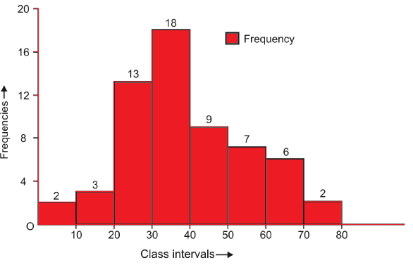
Histogram is similar to a bar diagram which represents a frequency distribution with continuous classes. The width of all bars is equal to class interval. Each rectangle is joined with the other so as to give a continuous picture.

The class-boundaries are located on the horizontal axis. If the class-intervals are of equal size, the heights of the rectangles will be proportional to the classfrequencies themselves. If the class-intervals are not of equal size, the heights of the rectangles will be proportional to the ratios of the frequencies to the width of the corresponding classes.

Example:

Frequency Polygon

Another method of presenting a frequency distribution graphically other than histogram is to use a frequency polygon. In order to draw the graph of a frequency polygon, first of all the mid values of all the class intervals and the corresponding frequencies are plotted as points with the help of the rectangular co-ordinate axes. Secondly, we join these plotted points by line segments. The graph thus obtained is known as frequency polygon, but one important point to keep in mind is that whenever a frequency polygon is required we take two imaginary class intervals each with frequency zero, one just before the first class interval and other just after the last class interval. Addition of these two class intervals facilitate the existence of the property that

Area under the polygon = Area of the histogram

For example, if we take the frequency distribution as given in Table 15.2 then, we have to first plot the points (5, 2), (15, 3), …, (75, 2) on graph paper along with the horizontal bars. Then we join the successive points (including the mid points of two imaginary class intervals each with zero frequency) by line segments to get a frequency polygon. The frequency polygon for frequency distribution given in Table of above example:

Example 1: Draw a frequency polygon for the following frequency distribution:

Sol:

Frequency Curve

Let us try to explain the concept theoretically. Suppose we draw a sample of size n from a large population. Frequency curve is the graph of a continuous variable. So theoretically continuity of the variable implies that whatever small class interval we take there will be some observations in that class interval. That is, in this case there will be large number of line segments and the frequency polygon tends to coincides with the smooth curve passing through these points as sample size (n) increases. This smooth curve is known as frequency curve.

Draw frequency polygon and frequency curve for the following frequency distribution.

Sol.:

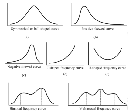
Some important types of frequency curves are given which are generally obtained in the graphical presentations of frequency distributions. That is, symmetrical, positively skewed, negatively skewed, J shaped, U shaped, bimodal and multimodal frequency curves.

Key takeaways:

1. In qualitative classification, data are classified on the basis of some attributes or qualitative characteristics such as sex, colour of hair, literacy, religion, etc.
2. A frequency distribution in which the information is distributed in different classes on the basis of a discrete variable is known as discrete frequency distribution.
3. A distribution in which the information is distributed in different classes on the basis of a continuous variable is known as continuous frequency distribution.
4. A relative frequency corresponding to a class is the ratio of the frequency of that class to the total frequency. The corresponding frequency distribution is called relative frequency distribution.
5. The cumulative frequency of a class is the total of all the frequencies up to and including that class.
6. 

1.8 Population, sample, parameter

Sampling distribution of a statistic is the theoretical probability distribution of the statistic which is easy to understand and is used in inferential or inductive statistics. A statistic is a random variable since its value depends on observed sample values which will differ from sample to sample. Whereas its particular value depends on a given set of sample values. Thus determination of sampling distribution of a statistic is essentially a mathematical problem.

Statistical methods are used to study a process by analyzing the data, discrete or continuous, recorded as either numerical value or a descriptive representation to improve the “quality” of the process. Thus statistician is mainly concerned with the analysis of data about the characteristics of persons or objects or observations.

POPULATION AND SAMPLE

Population is the set or collection or totality of objects, animate or inanimate, actual or hypothetical, under study. Thus mainly population consists of sets of numbers, measurements or observations which are of interest.

Size

Size of the population N is the number of objects or observations in the population.

Population is said to be finite or infinite depending on the size N being finite or infinite.

Since it is impracticable or uneconomical or time consuming to study the entire population, a finite subset of the population known as sample is studied.

Size of the sample is denoted by n. Sampling is the process of drawing samples from a given population.

Large sampling

If n ≥ 30, the sampling is said to be large sampling

Small sampling

If n < 30, the sampling is said to be small sampling or exact sampling

Statistical Inference

Statistical inference or inductive statistics deals with the methods of drawing (arriving at) valid or logical generalizations and predictions about the population using the information contained in the sample alone, with an indication of the accuracy of such inferences

Parameters

Statistical measures or constants obtained from the population are known as population parameters or simply parameters.

Example: Population mean, population variance. Similarly, statistical quantities computed from sample observations are known as sample statistics or briefly “statistics”. Thus parameters refer to population while statistics refer to sample.

Examples: sample mean, sample variance etc.

Notation

μ, σ, p represent the population mean, population standard deviation, population proportion. Similarly, X, s, P denote sample mean, sample s.d., sample proportion.

Population f(x)

Population f (x) is a population whose probability distribution is f (x).

Example: If f (x) is binomial, Poisson or normal, then the corresponding population is known as binomial population, Poisson population or normal population. Since the samples must be representative of the population, sampling should be random.

Random sampling is one in which each member of the population has equal chances or probability of being included in the sample. In sampling with replacement, each member of the population may be chosen more than once, since the member is replaced in the population.

Thus sampling from finite population with replacement can be considered theoretically as sampling from infinite population. Whereas, in sampling without replacement, an element of the population can not be chosen more than once, as it is not replaced.

Key takeaways:

1. Population is the set or collection or totality of objects, animate or inanimate, actual or hypothetical, under study.
2. Size of the population N is the number of objects or observations in the population.
3. Population is said to be finite or infinite depending on the size N being finite or infinite.
4. If n ≥ 30, the sampling is said to be large sampling
5. If n < 30, the sampling is said to be small sampling or exact sampling

References:

1. E. Kreyszig, “Advanced Engineering Mathematics”, John Wiley & Sons, 2006.

2. P. G. Hoel, S. C. Port and C. J. Stone, “Introduction to Probability Theory”, Universal Book Stall, 2003.

3. S. Ross, “A First Course in Probability”, Pearson Education India, 2002.

4. W. Feller, “An Introduction to Probability Theory and its Applications”, Vol. 1, Wiley, 1968.

5. N.P. Bali and M. Goyal, “A text book of Engineering Mathematics”, Laxmi Publications, 2010.

6. B.S. Grewal, “Higher Engineering Mathematics”, Khanna Publishers, 2000.

7. T. Veerarajan, “Engineering Mathematics”, Tata McGraw-Hill, New Delhi, 2010.

8. BV ramana mathematics.