Unit 5
Binary Trees
Binary Tree
A binary tree is a special cas eof tree in which no node of a tree can have degree more than two.
Definition of Binary Tree:
A binary tree is made of nodes, where each node contains a "left" pointer, a "right" pointer, and a data element. The "root" pointer points to the topmost node in the tree. The left and right pointers recursively point to smaller "subtrees" on either side. A null pointer represents a binary tree with no elements -- the empty tree.
The formal recursive definition is A binary tree is either empty (represented by a null pointer), or is made of a single node, where the left and right pointers (recursive definition ahead) each point to a binary tree.
Example of Binary Tree:
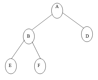
Fig.Example of Binary Tree
Types of Binary Tree,
1. Left Skewed Binary Tree:
2. Right Skewed Binary Tree:
1. Left Skewed Binary Tree:
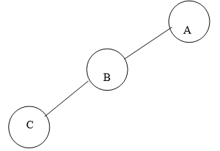
Fig. 4.6 Example of Left Skewed Binary Tree
In this tree, every node is having only Left sub tree.
2. Right Skewed Binary Tree:

A
B
C
Fig. Example of Right Skewed Binary Tree
In this tree, every node is having only Right sub tree.
Full or strict Binary Tree:
It is a binary tree of depth K having 2k-1 nodes.
For k=3, number of nodes=7
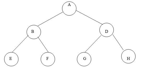
Fig. Example of strict Binary Tree
Complete Binary Tree:
It is a binary tree of depth K with N nodes in which these N nodes can be numbered sequentially from 1 to N.
Since a binary tree is an ordered tree and has levels, it is convenient to assign a number to each node.
Suppose for K=3:
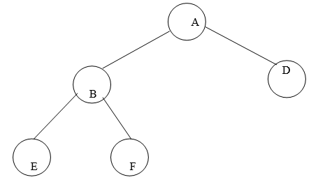
Fig. Example of Complete Binary Tree
The nodes can be numbered sequentially like:
Node number | Node |
1 | A |
2 | B |
3 | D |
4 | E |
5 | F |
Fig. Representation of Complete Binary Tree
Consider another example of binary tree:
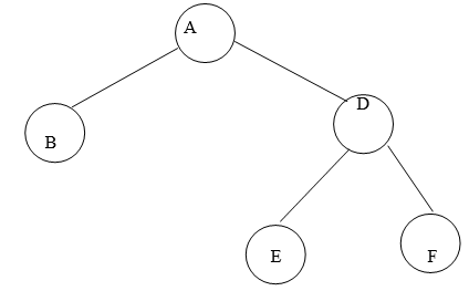
Fig. 4.11 Example of Non Complete Binary Tree
If we try to give numbers to nodes it would appear like:
Node number | Node |
1 | A |
2 | B |
3 | D |
4 | - |
5 | - |
6 | E |
7 | F |
Fig. 4.12 Representation of Non Complete Binary Tree
Here nodes cannot be numbers sequentially, so this kind of tree cannot be called as a complete binary tree
Binary Search Tree
We now turn our attention to search tress: Binary Search tress in this chapter and AVL Trees in next chapter. As seen in previous chapter, the array structure provides a very efficient search algorithm, the binary search, but it is inefficient for insertion and deletion algorithms. On the other hand, linked list structure provides efficient insertion and deletion algorithms but it is very inefficient for search algorithm. So what we need is a structure that provides efficient insertion, deletion as well as search algorithms.
Basic Concept:
A Binary Search Tree is a binary tree with the following properties:
1. It may be empty and every node has an identifier.
2. All nodes in left subtree are less than the root.
2. All nodes in right subtree are greater than the root.
4. Each subtree is itself a BST.
Examples of BST:
Valid BSTs:
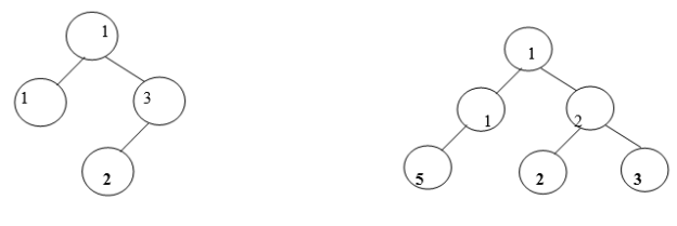
Fig. Examples of Valid BSTs
Invalid BSTs:

Fig.Examples of Invalid BSTs
Examine the BSTs in Fig.4.2. The first tree, Fig.4.2 (a) breaks the second rule: The left node 30 is greater than that of its root node 20. The second tree, Fig.4.2 (b) breaks the third rule: The right node 20 is less than that of its root node 50. The third tree, Fig.4.2 (c) breaks the second rule: The left node 25 is greater than that of its root node 10. It also breaks the third rule: The right node 08 is less than that of its root node 15.
Threaded Binary Tree
Binary trees, including binary search trees and their variants, can be used to store a set of items in a particular order. For example, a binary search tree assumes data items are ordered and maintain this ordering as part of their insertion and deletion algorithms. One useful operation on such a tree is traversal: visiting the items in the order in which they are stored .A simple recursive traversal algorithm that visits each node of a BST is the following. Assume t is a pointer to a node, or NULL.
Algorithm traverse_tree (root):
Input: a pointer root to a node (or NULL.)
If root = NULL, return.
Else
Traverse_tree (left-child (root))
Visit t
Traverse_tree (right-child (root))
The problem with this algorithm is that, because of its recursion, it uses stack space proportional to the height of a tree. If the tree is fairly balanced, this amounts to O(log n) space for a tree containing n elements.
One of the solutions to this problem is tree threading.
A threaded binary tree defined as follows:
"A binary tree is threaded by making all right child pointers that would normally be null point to the inorder successor of the node (if it exists), and all left child pointers that would normally be null point to the inorder predecessor of the node."
It is also possible to discover the parent of a node from a threaded binary tree, without explicit use of parent pointers or a stack. This can be useful where stack space is limited, or where a stack of parent pointers is unavailable (for finding the parent pointer via DFS).
Inorder Threaded Binary Tree:
In inorder threaded binary tree, left thread points to the predecessor and right thread points to the successor.
Types Inorder Threaded Binary Tree:
Right Inorder Threaded Binary Tree.
In this type of TBT, only right threads are shown which points to the successor.
Left Inorder Threaded Binary Tree.
In this type of TBT, only left threads are shown which points to the predecessor.
For TBT it is not necessary that the tree must be BST, it can be applied to general tree.
Example: Draw inorder TBT for following data:
10, 8, 1 5, 7, 9, 12, 18
Solution:
Step 1: The general for given data is:
1
8 1
7 9 1 1
Step 2: Write inorder sequence for the above tree:
7, 8, 9, 10, 12, 15, 18
Step 3: Make groups containing three nodes per group like:


 7 8 9 9 10 12 12 15 18
Step 4: It means right thread of 7 point to 8 provided that 7 node is not having right link, means right link of 7 is NULL and thread is pointing in bottom-up direction and not in top to bottom .
Left thread of 7 and Right thread of 18 will point to head node.
Step 5: Draw TBT with right and left threads.

Head Node
Left Inorder Threaded Binary Tree:

Right Inorder Threaded Binary Tree:

Introduction
A tree data structure can be defined recursively (locally) as a collection of nodes (starting at a root node), where each node is a data structure consisting of a value, together with a list of references to nodes (the "children"), with the constraints that no reference is duplicated, and none points to the root.
Definition of TREE:
A tree is defined as a set of one or more nodes T such that:
There is a specially designed node called root node
The remaining nodes are partitioned into N disjoint set of nodes T1, T2,…..Tn, each of which is a tree.
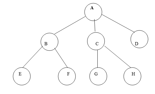
Fig. 4.1 Example of tree
In above tree A is Root.
Remaining nodes are partitioned into three disjoint sets:
{B, E, F}, {C, G, H}, {D}.
All these sets satisfies the properties of tree.
Some examples of TREE and NOT TREE

Each linear list is trivially a tree

Not a tree: cycle A→A
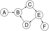
Not a tree: cycle B→C→E→D→B

Not a tree: two non-(connected parts, A→B and C→D→E
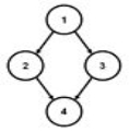
Not a tree: undirected cycle 1-2-4-3
Fig. Examples of tree and no tree
Tree Terminologies
- Root – The top node in a tree.
- Parent – The converse notion of child.
- Siblings – Nodes with the same parent.
- Descendant – a node reachable by repeated proceeding from parent to child.
- Ancestor – a node reachable by repeated proceeding from child to parent.
- Leaf – a node with no children.
- Internal node – a node with at least one child.
- External node – a node with no children.
- Degree – number of sub trees of a node.
- Edge – connection between one node to another.
- Path – a sequence of nodes and edges connecting a node with a descendant.
- Level – The level of a node is defined by 1 + the number of connections between the node and the root.
- Height of tree –The height of a tree is the number of edges on the longest downward path between the root and a leaf.
- Height of node –The height of a node is the number of edges on the longest downward path between that node and a leaf.
- Depth –The depth of a node is the number of edges from the node to the tree's root node.
- Forest – A forest is a set of n ≥ 0 disjoint trees.
- Search − Searches an element in a tree.
- Insert − Inserts an element in a tree.
- Pre-order Traversal − Traverses a tree in a pre-order manner.
- In-order Traversal − Traverses a tree in an in-order manner.
- Post-order Traversal − Traverses a tree in a post-order manner.
Node
Define a node having some data, references to its left and right child nodes.
Struct node {
Int data;
Struct node *leftChild;
Struct node *rightChild;
};
Search Operation
Whenever an element is to be searched, start searching from the root node. Then if the data is less than the key value, search for the element in the left subtree. Otherwise, search for the element in the right subtree. Follow the same algorithm for each node.
Algorithm
Struct node* search(int data){
Struct node *current = root;
Printf("Visiting elements: ");
While(current->data != data){
If(current != NULL) {
Printf("%d ",current->data);
//go to left tree
If(current->data > data){
Current = current->leftChild;
} //else go to right tree
Else {
Current = current->rightChild;
}
//not found
If(current == NULL){
Return NULL;
}
}
}
Return current;
}
Insert Operation
Whenever an element is to be inserted, first locate its proper location. Start searching from the root node, then if the data is less than the key value, search for the empty location in the left subtree and insert the data. Otherwise, search for the empty location in the right subtree and insert the data.
Algorithm
Void insert(int data) {
Struct node *tempNode = (struct node*) malloc(sizeof(struct node));
Struct node *current;
Struct node *parent;
TempNode->data = data;
TempNode->leftChild = NULL;
TempNode->rightChild = NULL;
//if tree is empty
If(root == NULL) {
Root = tempNode;
} else {
Current = root;
Parent = NULL;
While(1) {
Parent = current;
//go to left of the tree
If(data < parent->data) {
Current = current->leftChild;
//insert to the left
If(current == NULL) {
Parent->leftChild = tempNode;
Return;
}
} //go to right of the tree
Else {
Current = current->rightChild;
//insert to the right
If(current == NULL) {
Parent->rightChild = tempNode;
Return;
}
}
}
}
}
Huffman’s Algorithm:
Huffman Codes:
Huffman coding is a simple data compression scheme.
Fixed-Length Codes
Suppose we want to compress a 100,000-byte data file that we know contains only the lowercase letters A through F. Since we have only six distinct characters to encode, we can represent each one with three bits rather than the eight bits normally used to store characters:
Letter | A | B | C | D | E | F | |
Codeword | 000 | 001 | 010 | 011 | 100 | 101 | |
This fixed-length code gives us a compression ratio of 5/8 = 62.5%.
Variable-Length Codes
What if we knew the relative frequencies at which each letter occurred? It would be logical to assign shorter codes to the most frequent letters and save longer codes for the infrequent letters. For example, consider this code:
Letter | A | B | C | D | E | F |
Frequency (K) | 45 | 13 | 12 | 16 | 9 | 5 |
Codeword | 0 | 101 | 100 | 111 | 1101 | 1100 |
Using this code, our file can be represented with
(45×1 + 13×3 + 12×3 + 16×3 + 9×4 + 5×4) × 1000 = 224 000 bits
Or 28 000 bytes, which gives a compression ratio of 72%. In fact, this is an optimal character code for this file (which is not to say that the file is not further compressible by other means).
Prefix Codes
Notice that in our variable-length code, no codeword is a prefix of any other codeword. For example, we have a codeword 0, so no other codeword starts with 0. And both of our four-bit code words start with 110, which is not a codeword. Such codes are called prefix codes. Prefix codes are useful because they make a stream of bits unambiguous; we simply can accumulate bits from a stream until we have completed a codeword. (Notice that encoding is simple regardless of whether our code is a prefix code: we just build a dictionary of letters to code words, look up each letter we're trying to encode, and append the code words to an output stream.) In turns out that prefix codes always can be used to achieve the optimal compression for a character code, so we're not losing anything by restricting ourselves to this type of character code.
When we're decoding a stream of bits using a prefix code, what data structure might we want to use to help us determine whether we've read a whole codeword yet?
One convenient representation is to use a binary tree with the code words stored in the leaves so that the bits determine the path to the leaf. In our example, the codeword 1100 is found by starting at the root, moving down the right sub tree twice and the left sub tree twice.
Huffman’s algorithm is used to build such type of binary tree.
Algorithm:
Arrange list in ascending order of frequencies.
Create new node with addition of frequencies of first two nodes.
Insert this new node into list and again sort it.
Repeat till only one value remains in the list.
Consider alphabets and their frequencies of occurrences are as:
Letter | A | B | C | D | E | F |
Frequency (K) | 45 | 13 | 12 | 16 | 9 | 5 |
Huffman Algorithm for above data will work like :
Step1: sort the list in ascending order
5 9 12 13 16 45
Step2: New node’s frequency=5+9=14
12 13 14 16 45
Step3: New node’s frequency=12+13=25
14 16 25 45
Step4: New node’s frequency=14+16=30
25 30 45
Step4: New node’s frequency=25+30=55
45 55
Step4: New node’s frequency=45+55=100
100
Final Huffman’s tree will be:

 100
100

 45[A] 55


 25 30
25 30

 12[C] 13[B] 14 16[D]
5 [F] 9 [E]