Module-1
Differential calculus-1
Polar curves-
Angle between the radius vector and tangent-
If  be the angle between the radius vector and the tangent at any point of the curve

Length of the perpendicular from pole on the tangent-
If p be the perpendicular from the pole on the tangent, then-
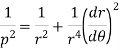
And

Note-
Polar sub-tangent is-

And polar sub-normal is-

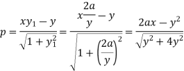
Example: Find out the angle of intersection of the curves 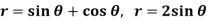
Sol.
We eliminate ‘r’ to find the point of intersection of the curves-
And
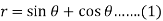
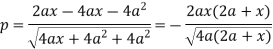
Then-
Or
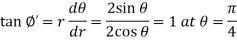
For (1)-
So that-
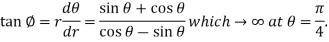
Thus

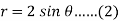
For equation (2)-

So that-
Thus

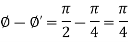
Therefore the angle of intersection of the curves-
Key takeaways-
- Polar sub-tangent is-

2. And polar sub-normal is-

Angle of intersection of two curves-
We follow the procedure given below to find out the angle 
- Find the point of intersection (P) of the curves by solving their equations.
- Find the value of dy/dx at P for the two curves (

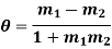
- Find angle


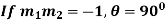
Note- If  then the curves cut orthogonally.
Pedal equation-
The relation between ‘p’ and ‘r’ is called pedal equation of the curve where ‘r’ is the radius vector of any point on the curve and ‘p’ be the length of the perpendicular from the pole on the tangent at that point.
Exampe-1: Find the pedal equation of the parabola 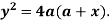
Sol.
Equation of the tangent of the parabola can be written as-
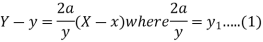
The perpendicular distance of this tangent from (0,0)-
Implying-
Or

Now-

Or

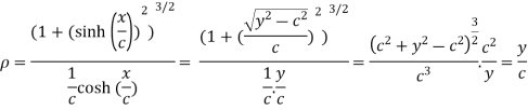
Therefore the pedal equation is-

Example: Find the pedal equation of the ellipse-

Sol.
Here we have-
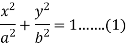
Equation of the tangent at (x, y) is-
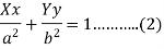
The length of perpendicular ‘p’ from (0, 0) on (2)-
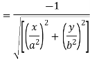
Or
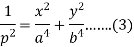
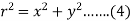
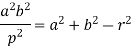
Also-
Put the value of  from (4) in (1), we get-

Then from (1)-

Now put these values of  in (3), we get-
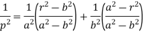
Or
Which is the required pedal equations.
Key takeaways-
- Angle of intersection of two curves-
2.  then the curves cut orthogonally.
Curvature
Let M be any point on the given curve and  be its neighborhood.
Let s be an arc of the curve at M and  s be the arc at
  shown in the figure and
  be an angle made by the tangent at point M and
  at the point
  of the curve. Then the infinitely small length of the arc M
 i.e.
i.e.  and angle made by the tangent between them is
  .
.
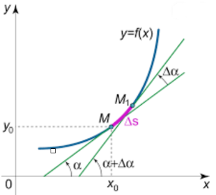
Then the curvature of the curve when M tends to  is
is 
i.e. the derivative of the angle made by the tangent to the curve with respect to the arc at that point.
The unit of curvature is radian per length.
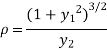
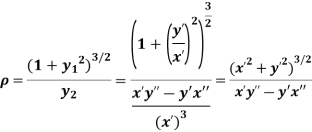
Radius of curvature: The radius of curvature is the reciprocal of the curvature of the curve at the point. It is denoted by  .
.

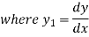
We know that slope is 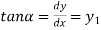
Or

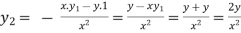
Differentiating both side with respect to x we get,

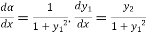
By chain rule 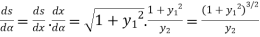
Hence
Example-1: Show that for a rectangular hyperbola ,
,  ?
?
Sol.
Given curve  .
.
Differentiating both side with respect to x.

Or  ……(i)
……(i)
Again differentiating with respect to x.
 using (i)
 ….(ii)
The radius of curvature is
Substituting values from (i) and (ii) we get
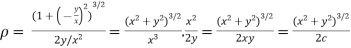 by given curve.
Hence  is proved.
Example2:
Find the radius of curvature at  of the catenary
 ?
?
Sol.
Given catenary  … (i)
… (i)
Differentiating (i) with respect to x.
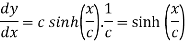
Also consider 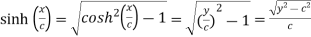
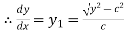 ….. (ii)
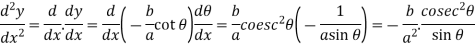
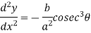
Again differentiating with respect to x , we get
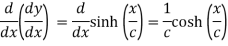
 ….(iii)
The radius of curvature is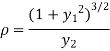
Substituting values from (i),(ii) and (iii) we get
Hence the radius of curvature at  is
is  .
.
Radius of Curvature in parametric form:
Let the co-ordinates be defined in the form of functions depend on one independent variable t.
Suppose 
We will calculate the values in term of variables depend on t.
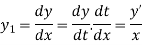
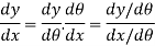
By chain rule we have
And
By
Example:
Find the radius of curvature at any point on
- Ellipse
 .
.
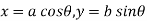
The parametric equation of the ellipse is given by
As we know by chain rule
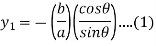
Hence
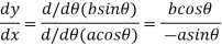
Or
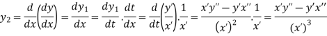
Again by chain rule we have
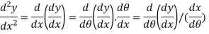
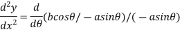
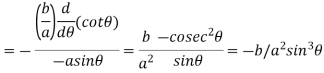
Hence 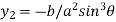 …..(ii)
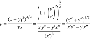
The radius of curvature is
Substituting values from (i), and (ii) we get
Newton’s formula for radius of curvature at origin:
- If x-axis is tangent to a curve at the origin, then
b. If y-axis is tangent to a curve at the origin, then
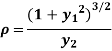
c. When the tangent is at the origin and neither on x-axis nor on y-axis then

Where .
.
Note: To find the tangent at the origin of the curve we will equate the lowest degree term in the equation to zero.
Example: Find the radius of curvature at the origin for
Sol.
Given curve is  ….(i)
….(i)
Equating lowest degree term to zero we get
 ..(ii)
 Tangent at the origin is on the x-axis.
Dividing (i) by y , we get
The radius of curvature at the origin on the x-axis is  and using (ii)
 .
.
Example: Find the radius of curvature at the origin for- 
Given curve  …(i)
…(i)
Equating lowest degree term to zero we get
 ..(ii)
 Tangent at the origin is on the y-axis.
Dividing (i) by x, we get
The radius of curvature at the origin on the x-axis is  and using (ii)
 .
.
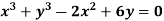
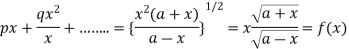
Example: Find the radius of curvature at the origin for-
Sol. Given curve 
Or 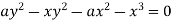 …(i)
…(i)
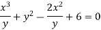
Equating lowest degree term to zero we get
 ..(ii)
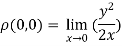
 Tangent at the origin is neither on x-axis nor on y-axis.
Putting in (i),  where
where 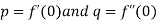 .
.
Where 
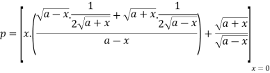
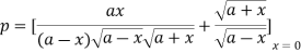
Hence 
Again 
 .
.
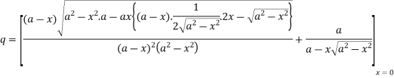
When the tangent is at the origin and neither on x-axis nor on y-axis then
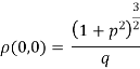
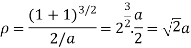
Substituting the values in p and q we get,
Key takeaways-
- Radius of curvature: The radius of curvature is the reciprocal of the curvature of the curve at the point. It is denoted by
 .
.
2. Radius of Curvature in parametric form:
3. To find the tangent at the origin of the curve we will equate the lowest degree term in the equation to zero.
Centre of curvature-
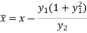
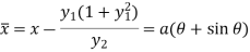
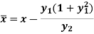
Centre of curvature at any point P (x, y) on the curve y = f(x) is given by-
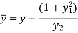
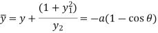
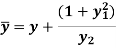
And
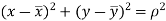
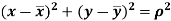
Circle of curvature at P-
Example: Find the coordinates of the centre of curvature at any point of the cycloid-

Sol.
Here we have-
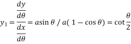
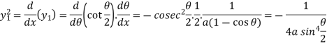
Then centre of curvature-
On putting the above value in formulas, we get-
Evolutes and involutes-
Definition- The locus of centres of curvature of a given curve is called the evolute of that curve.
The locus of the center of curvature C of a variable point P on a curve is called the evolute of the curve and the curve itself is called involute of the evolute.
Evolute is nothing but an equation of the curve.
Method to find the evolute-
1. If a curve equation is given and we need to prove left hand side is equal to right hand side (L.H.S = R.H.S), then
First of all find the curvature C(X,Y), where
And
Then take left hand side and put X in place of x and Y in place of y.
2. When the curve is given and we need to find the evolute, then-
Find the curvature first and then re-write as x in terms of X and y in terms of Y and then put in the given curve
Properties of envelope and evolute-
1. The normal at any point of a curve is a tangent to its evolute touching at the corresponding centre of curvature.
2. The evolute is one only but there can be infinite involutes.
3. The difference between the radii of curvature at two points of a curve is equal to the length of the arc of the evolute between the two corresponding points.
Example: Prove that the evolute of parabola  is given by
Sol. It is given that-

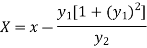
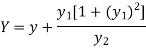
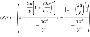
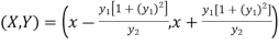
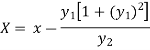
If (X,Y) are the coordinates of the centre of curvature at any point P(x , y) on the curve y = f(x), then X and Y are given as-
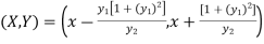 …………….. (1)
Now consider the equation of parabola (given)

On differentiating w.r.t x-
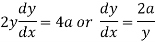
Again differentiating w.r.t.x-
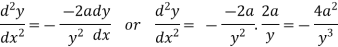
Put these derivatives in (1), we get-
Now consider X,
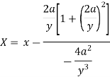
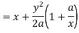

Here we get-

Now consider,
Here we get-

Now
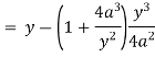
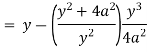
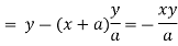
Taking L.H.S of 
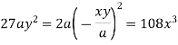
Taking R.H.S of 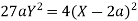

Hence proved.
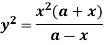
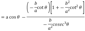
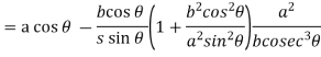
Example: Find the evolute of the ellipse  .
.
Sol. It is given that-

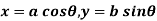
The parametric equations are 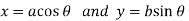
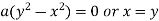
Now,
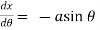 and
and
So that-
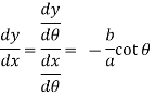
Which gives,
Co-ordinates of centre of curvature are (X , Y),
 …………….. (1)
Consider X,
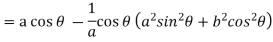
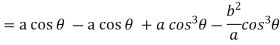
We get-
Now consider Y,
So that we get-
Eliminating  from X and Y, we get,
 and
and
We know that 
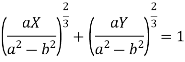
Which gives on solving-
Which is the required evolute.
Envelop of a family of curves-
Let us consider a family of plane curves (single-parameter) which is defined by the following equation-

Here C is a parameter.
Then the envelope of this family of curves is a curve such that at every point it touches one of the curves of the family.
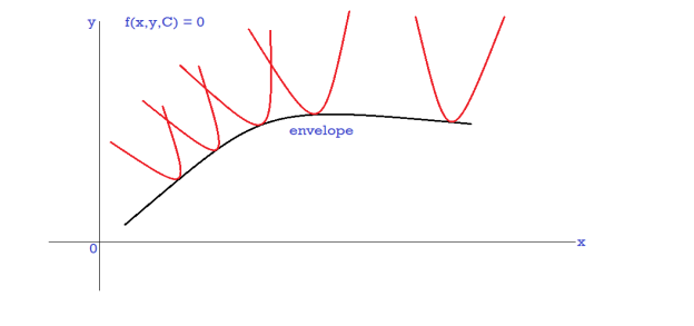
In the figure black curve is an envelope.
Note-
1. Envelope- A curve which touches each member of a family of curves is called envelope of that family of curves.
2. Envelope of a family of curves-
The locus of the ultimate points of interaction of consecutive members of a family of curve is called the envelope of the family of curves.
Example:
Find the envelope of  , where m is the parameter and A, B and C are function x and y.
Sol. It is given that-
 ………………….. (1)
Now differentiate equation (1) with respect to ‘m’,
We get-
 , gives

Put these values in equation (1)-
Which gives-

Which is the required envelope.
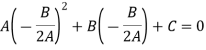
Example: Find the envelope of the family of  , where
  is the parameter.
Sol. It is given that-
 ………….. (1)
Now differentiate equation (1) with respect to ‘ ’,
’,
We get-
 ………………… (2)
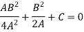
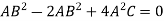
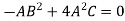
Eliminate  from both equations-
We get-
 And
And 
Put these values in (1) -

On squaring both sides, we get-

Which is the required envelope.
Example: Find the envelope of the family of straight lines  , where ‘m’ is the parameter.
Sol. It is given that-
Which can be written as-

 , which is a quadratic equation.
Here the value of coefficients of the quadratic equation-

The condition for envelope in case of a quadratic equation is-


So that the envelope is 
Key takeaways-
- Centre of curvature-
And
2. Circle of curvature at P-
3. Envelope- A curve which touches each member of a family of curves is called envelope of that family of curves.
4. Envelope of a family of curves-
The locus of the ultimate points of interaction of consecutive members of a family of curve is called the envelope of the family of curves.
References:
- C.Ray Wylie, Louis C.Barrett : "Advanced Engineering Mathematics", 6th Edition, 2. McGraw-Hill Book Co., New York, 1995.
- James Stewart : “Calculus -Early Transcendentals”, Cengage Learning India Private Ltd., 2017.
- B.V.Ramana: "Higher Engineering Mathematics" 11th Edition, Tata McGraw-Hill, 2010.
- Srimanta Pal & Subobh C Bhunia: “Engineering Mathematics”, Oxford University Press, 3rd Reprint, 2016.
- Gupta C.B., Singh S.R. And Mukesh Kumar: “Engineering Mathematics for Semester I & II”, Mc-Graw Hill Education (India) Pvt.Ltd., 2015.


