Module-4
Ordinary differential equations of first order
Definition-
An exact differential equation is formed by differentiating its solution directly without any other process,
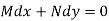
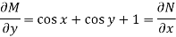
Is called an exact differential equation if it satisfies the following condition-

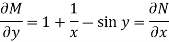
Here  is the differential co-efficient of M with respect to y keeping x constant and
  is the differential co-efficient of N with respect to x keeping y constant.
Step by step method to solve an exact differential equation-
1. Integrate M w.r.t. x keeping y constant.
2. Integrate with respect to y, those terms of N which do not contain x.
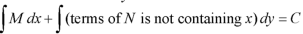
3. Add the above two results as below-

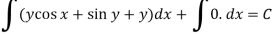
Example-1: Solve 
Sol.
Here M = 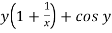 and N =
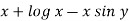
Then the equation is exact and its solution is-
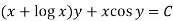
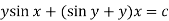
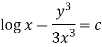
Example-2: Solve-
Sol. We can write the equation as below-

Here M = 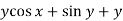 and N =
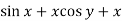
So that-
The equation is exact and its solution will be-

Or
Example-3: Determine whether the differential function ydx –xdy = 0 is exact or not.
Solution. Here the equation is the form of M(x , y)dx + N(x , y)dy = 0
But, we will check for exactness,


These are not equal results, so we can say that the given diff. Eq. Is not exact.
Equation reducible to exact form-
1. If M dx + N dy = 0 be an homogenous equation in x and y, then 1/ (Mx + Ny) is an integrating factor.
Example: Solve-

Sol.
We can write the given equation as-

Here,
M = 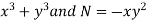
Multiply equation (1) by  we get-
This is an exact differential equation-
2. I.F. For an equation of the type 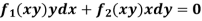
IF the equation Mdx + Ndy = 0 be this form, then 1/(Mx – Ny) is an integrating factor.
Example: Solve-

Sol.
Here we have-
Now divide by xy, we get-


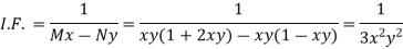
Multiply (1) by  , we get-
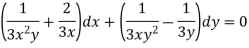
Which is an exact differential equation-
3. In the equation M dx + N dy = 0,
(i) If  be a function of x only = f(x), then
  is an integrating factor.
(ii) If  be a function of y only = F(x), then
  is an integrating factor.
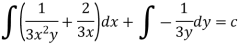
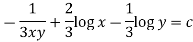
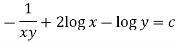
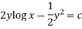
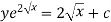
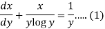
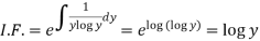
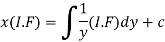
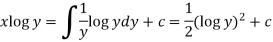
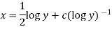
Example: Solve-

Sol.
Here given,

M = 2y and N = 2x log x - xy
Then-
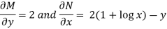
Here,
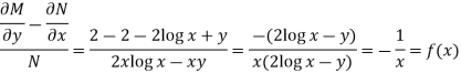
Then,
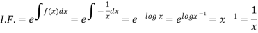
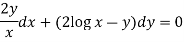
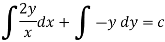
Now multiplying equation (1) by 1/x, we get-
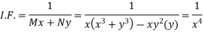
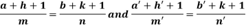
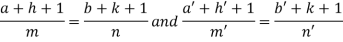
4. For the following type of equation-

An I.F. Is 
Where-
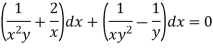
Example: Solve-

Sol.
We can write the equation as below-

Now comparing with-

We get-
a = b = 1, m = n = 1, a’ = b’ = 2, m’ = 2, n’ = -1
I.F. = 
Where-
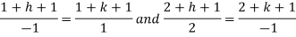
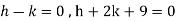
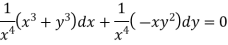
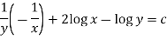
On solving we get-
h = k = -3

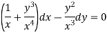
Multiply the equation by  , we get-
It is an exact equation.
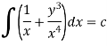
So that the solution is-
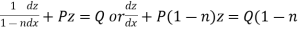
Bernoulli’s equation-
The equation
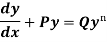
Is reducible to the Leibnitz’s linear equation and is usually called Bernoulli’s equation.
Working procedure to solve the Bernoulli’s linear equation-
Divide both sides of the equation -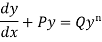
By , so that
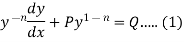
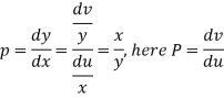
Put  so that
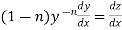
Then equation (1) becomes-
 )
)
Here we see that it is a Leibnitz’s linear equations which can be solved easily.
Example: Solve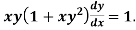
Sol.
We can write the equation as-
On dividing by  , we get-
Put  so that
Equation (1) becomes,
Here,
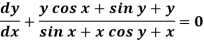
Therefore the solution is-
Or
Now put 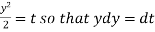
Integrate by parts-
Or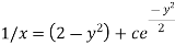
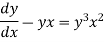
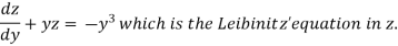
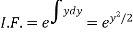
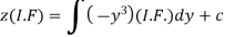
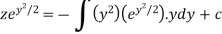
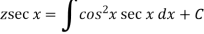
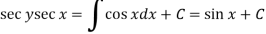
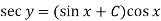
Example: Solve 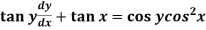
Sol. Here given,
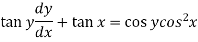
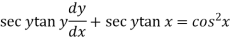
Now let z = sec y, so that dz/dx = sec y tan y dy/dx
Then the equation becomes-
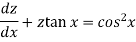
Here,
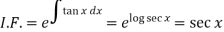
Then the solution will be-
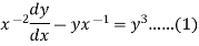
Example: Solve- 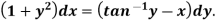
Sol. Here given-
We can re-write this as-
Which is a linear differential equation-
The solution will be-
Put 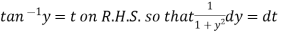

“When every curve of either family cuts each curve of other family at right angle in the two families of curve, then they are orthogonal trajectories of each other.”
Ex. 1. The line of heat flow is perpendicular to isothermal curve.
Steps to find orthogonal trajectories of curves-:
1. Differentiate the equation of the curve and find the differential equation as below-
f = 0
= 0
2. Replace  by
by 
3. Solve the differential equation of the orthogonal trajectories,
f = 0
= 0
Self-orthogonal - if the family of orthogonal traj. Is same as the family of curves, then it is called self-orthogonal.
Example: if the family of curves is xy = c , then find its orthogonal trajectory.
Sol. First we will differentiate the given equation with respect to x,
We get,
y + x  = 0
= 0
 =
= 
Replace  by
by 
 =
= 
 =
= 
We get,
Ydy = x dx
Now integrate this equation, we get
 =
=  + c
+ c
y² - x² = 2c. Ans.
Example: find the orthogonal trajectory of the family of curves x² - y² = c
Sol. Here we will follow same procedure as we did in above example,
Diff. The given equation w.r.t. x, we get
2x – 2y = 0
= 0
 =
= 
Replace  by
by 
 =
= 
 = -
= - 
Ydy = - xdx
Now integrate the above eq.
 =
=  + c
+ c
On solving we get,
x² + y² = 2c.
Newton’s law of cooling-
According to Newton’s law of cooling, the temperature of any body changes at a rate which is proportional to the difference in temperature between that of surrounding medium and that of the body itself.
If at any time ‘t’,  is the temperature of the surroundings and
  is the temperature of the body itself, then-
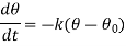
Here k is the constant.
Example: If a body which is at the temperature of  cools down to
  within 20 minutes. The temperature of the air is
  .
.
Find that what will be the temperature of the body after 40 min from its original temperature?
Sol.
Suppose  be the temperature of the body at time ‘t’ then-
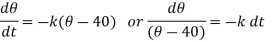
Here k is the constant.
On integrating, we get-
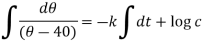
‘c’ is the constant
Or
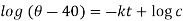
Or
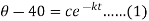
When t = 0,  and when t = 20 then
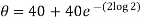
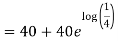
So that-  and
and
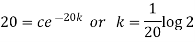
Then equation (1) becomes-
Now, when t = 40 minutes, then-

2. RL circuit – Let us consider a resister R, an inductor L and a capacitor C which are connected in a series ,
Let ϵ(t) = ϵ’cosωt is an electromotive force to the circuit,
The equations for the voltage drops across a capacitor , a register and an inductor are
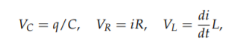
Where C is the capacitance, R is the resistance and L is the inductance , q is the charge and i is the current
We know that from Kirchhof’s law,
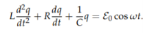
This is the second order non- homogeneous differential equation with constant coefficients.
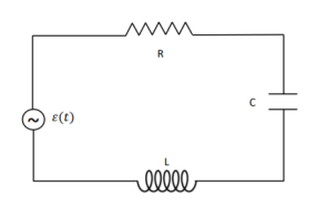
Diagram for RLC circuit
A differential equation of the form

Is called linear differential equation.
It is also called Leibnitz’s linear equation.
Here P and Q are the function of x
Working rule
(1)Convert the equation to the standard form 
(2) Find the integrating factor.
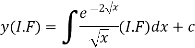
(3) Then the solution will be y(I.F) = 
Example-1: Solve-
Sol. We can write the given equation as-
So that-
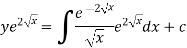
I.F. = 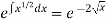
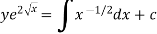
The solution of equation (1) will be-
Or
Or
Or
Example-2: Solve-

Sol.
We can write the equation as-
We see that it is a Leibnitz’s equation in x-
So that-
Therefore the solution of equation (1) will be-
Or
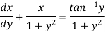
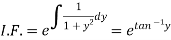
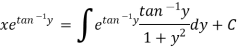
Example-3: Solve
Solution: here we have,
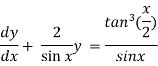
Which is the linear form,
Now,
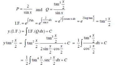
Put tan so that
  sec²
sec² dx = dt, we get
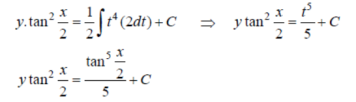
Which is the required solution
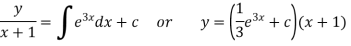
Example-4: Solve-
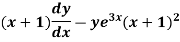
Sol.
Here we have-
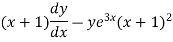
Divide this by (x + 1), we get-
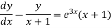
Which is the Leibnitz’s equation-
Here-

And
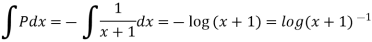
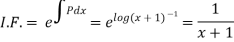
Integrating factor-
The solution will be-
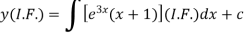
Or
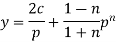
Equation solvable for p-
Example- Solve-

Sol. Here we have-

Or


On integrating, we get-
Equation solvable for y-
Steps-
First- differentiate the given equation w.r.t. x.
Second- Eliminate p from the given equation, then the eliminant is the required solution.
Example: Solve 
Sol.
Here we have-
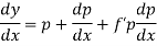
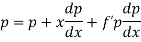
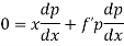
Now differentiate it with respect to x, we get-
Or
This is the Leibnitz’s linear equation in x and p, here
Then the solution of (2) is-
Or
Or
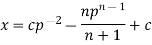
Put this value of x in (1), we get
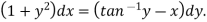
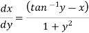
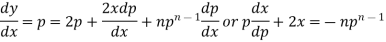
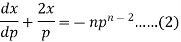
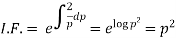
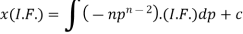
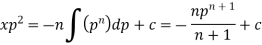
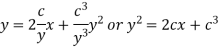
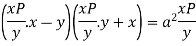
Equation solvable for x-
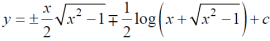
Example: Solve-
Sol. Here we have-
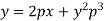
On solving for x, it becomes-

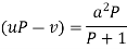
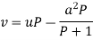
Differentiating w.r.t. y, we get-
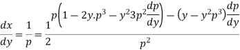
Or
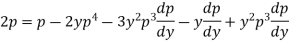
On solving it becomes
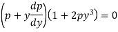
Which gives-

Or

On integrating

Thus eliminating from the given equation and (1), we get
Which is the required solution.
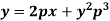
Clairaut’s equation-
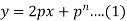
An equation
y = px + f(p) ...... (2)
Is known as Clairaut’s equation.
Differentiating (1) w.r.t. x, we get-

Put the value of p in (1) we get-
y = ax + f(a)
Which is the required solution.
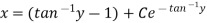
Example: Solve-
Sol.
Put 
So that-
Then the given equation becomes-
Or
Or
Which is the Clairaut’s form.
Its solution is-

i.e.
References:
- C.Ray Wylie, Louis C.Barrett : "Advanced Engineering Mathematics", 6th Edition, 2. McGraw-Hill Book Co., New York, 1995.
- James Stewart : “Calculus -Early Transcendentals”, Cengage Learning India Private Ltd., 2017.
- B.V.Ramana: "Higher Engineering Mathematics" 11th Edition, Tata McGraw-Hill, 2010.
- Srimanta Pal & Subobh C Bhunia: “Engineering Mathematics”, Oxford University Press, 3rd Reprint, 2016.
- Gupta C.B., Singh S.R. And Mukesh Kumar: “Engineering Mathematics for Semester I & II”, Mc-Graw Hill Education (India) Pvt.Ltd., 2015.


