Unit 1
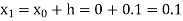
Numerical methods
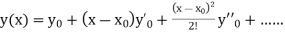
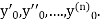
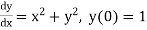
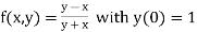
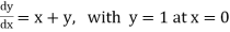
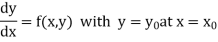
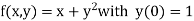
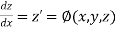
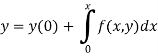
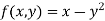
The general first order differential equation
|

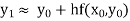
With the initial condition  …(2)
…(2)
In general, the solution of first order differential equation in one of the two forms:
a) A series for y in terms of power of x, from which the value of y can be obtained by direct solution.
b) A set of tabulated values of x and y.
The case (a) is solved by Taylor’s Series or Picard method whereas case (b) is solved by Euler’s, Runge Kutta Methods etc.
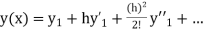
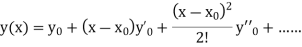
Taylor’s Series Method:
The general first order differential equation
With the initial condition Let
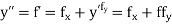
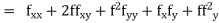
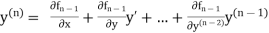
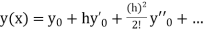
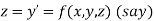
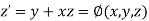
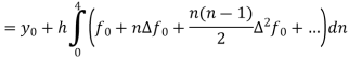
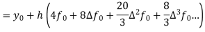
If the values of And other higher derivatives of y. The method can easily be extended to simultaneous and higher –order differential equations. In general, Putting
|


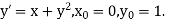
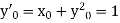
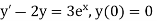
Example1: Solve
using Taylor’s series method and compute |


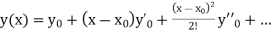
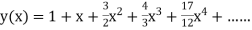
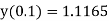
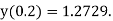
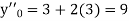
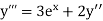
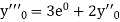
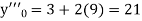
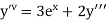
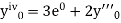
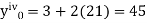
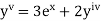
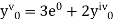
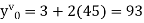
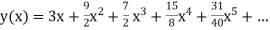
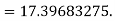
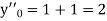
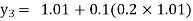
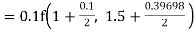
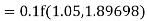
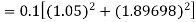
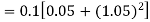
Here Differentiating, we get The Taylor’s series at At At |


Example2: Using Taylor’s series method, find the solution of
|
At 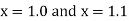 ?
?
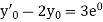
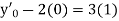
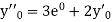
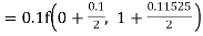
Here At Differentiating, we get The Taylor’s series at At At |


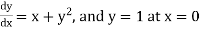
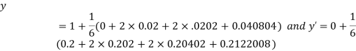
Example3: Solve
numerically, start from |


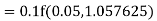
Here We have Differentiating, we get The Taylor’s series at Or Here The Taylor’s series |


Key takeaways
- The Taylor’s series for
 around
  is given by
|
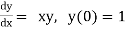
Euler’s method:
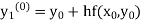
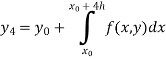
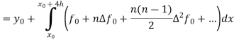
In this method the solution is in the form of a tabulated values
Integrating both side of the equation (i) we get
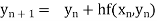
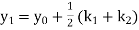
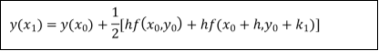
Assuming that In general formula Error estimate for the Euler’s method |


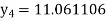
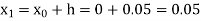
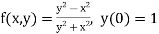
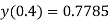
Example1: Use Euler’s method to find y(0.4) from the differential equation
|
Given
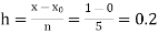
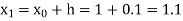
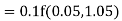
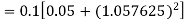
Equation Here We break the interval in four steps. So that By Euler’s formula For n=0 in equation (i) we get For n=1 in equation (i) we get For n=2 in equation (i) we get For n=3 in equation (i) we get Hence y(0.4) =1.061106. |


Example2: Using Euler’s method solve the differential equation for y at x=1 in five steps
|
Given
equation Here No. of steps n=5 and so that So that Also By Euler’s formula For n=0 in equation (i) we get For n=1 in equation (i) we get For n=2 in equation (i) we get For n=3 in equation (i) we get For n=4 in equation (i) we get Hence
|


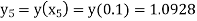
Example3: Given
|

with the initial condition y=1 at x=0.Find y for x=0.1 by Euler’s method (five steps).
Given
equation is Here No. of steps n=5 and so that So that Also By Euler’s formula For n=0 in equation (i) we get For n=1 in equation (i) we get For n=2 in equation (i) we get For n=3 in equation (i) we get For n=4 in equation (i) we get Hence |


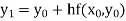
Modified Euler’s Method:
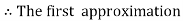
Instead of approximating  as in Euler’s method. In the modified Euler’s method we have the iteration formula
|

Where  is the nth approximation to
  .The iteration started with the Euler’s formula
|
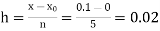
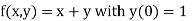
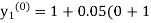
Example1: Use modified Euler’s method to compute y for x=0.05. Given that
|
Result correct to three decimal places.
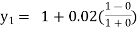
Given
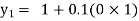
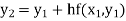
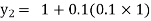
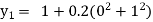
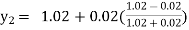
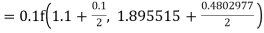
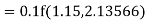
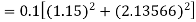
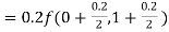
equation Here Take h = By modified Euler’s formula the initial iteration is The iteration formula by modified Euler’s method is For n=0 in equation (i) we get Where For n=1 in equation (i) we get
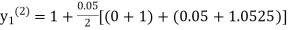
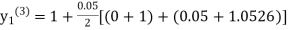
For n=3 in equation (i) we get Since third and fourth approximation are equal. Hence y=1.0526 at x = 0.05 correct to three decimal places. |


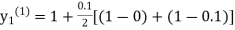
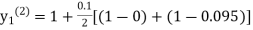
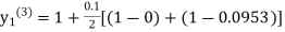
Example2: Using modified Euler’s method, obtain a solution of the equation
|

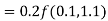
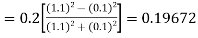
Given
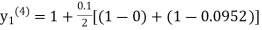
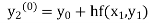
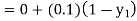
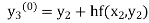
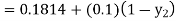
equation Here By modified Euler’s formula the initial iteration is The iteration formula by modified Euler’s method is For n=0 in equation (i) we get Where For n=1 in equation (i) we get For n=2 in equation (i) we get For n=3 in equation (i) we get Since third and fourth approximation are equal. Hence y=0.0952 at x=0.1 To calculate the value of By modified Euler’s formula the initial iteration is The iteration formula by modified Euler’s method is For n=0 in equation (ii) we get For n=1 in equation (ii) we get Since first and second approximation are equal. Hence y = 0.1814 at x=0.2 To calculate the value of By modified Euler’s formula the initial iteration is The iteration formula by modified Euler’s method is For n=0 in equation (iii) we get
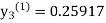
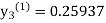
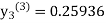
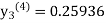
For n=1 in equation (iii) we get For n=2 in equation (iii) we get For n=3 in equation (iii) we get Since third and fourth approximation are same. Hence y = 0.25936 at x = 0.3 |


Key takeaways
- Euler’s method:
|


This method is more accurate than Euler’s method.
Consider the differential equation of first order
|
Let  be the first interval.
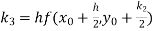
A second order Runge Kutta formula
|
Where |

 Rewrite as
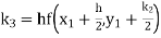
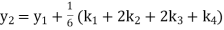
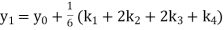
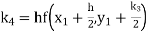
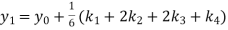
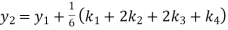
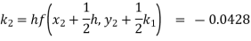
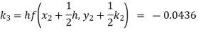
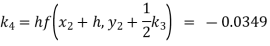
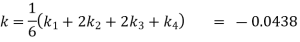
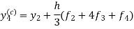
A fourth order Runge Kutta formula: Where |


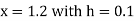
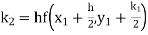
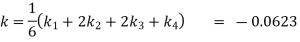
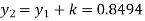
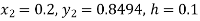
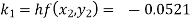
Example1: Use Runge Kutta method to find y when x=1.2 in step of h=0.1 given that
|
Given
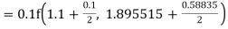
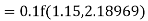
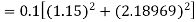
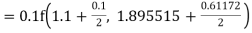
equation Here Also By Runge Kutta formula for first interval Again A fourth order Runge Kutta formula: To find y at A fourth order Runge Kutta formula: |


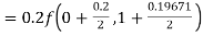
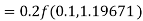
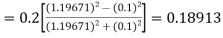
Example2: Apply Runge Kutta fourth order method to find an approximate value of y for x=0.2 in step of 0.1, if
|
Given
equation Here Also By Runge Kutta formula for first interval A fourth order Runge Kutta formula: Again A fourth order Runge Kutta formula: |


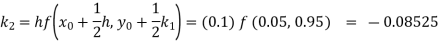
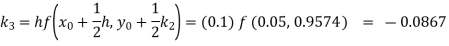
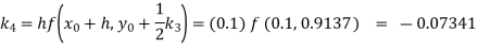
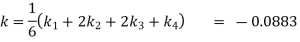
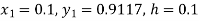
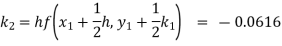
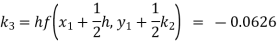
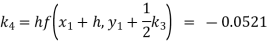
Example3: Using Runge Kutta method of fourth order, solve
|
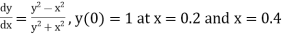
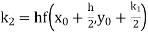
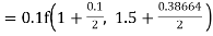
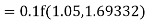
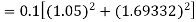
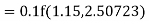
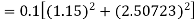
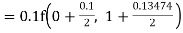
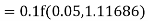
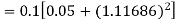
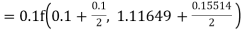
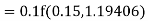
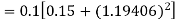
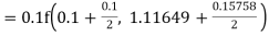
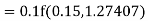
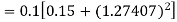
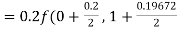
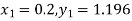
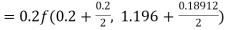
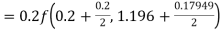
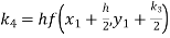
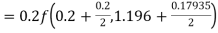
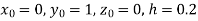
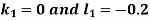
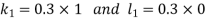
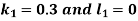
Given
equation Here Also By Runge Kutta formula for first interval A fourth order Runge Kutta formula: Hence at x = 0.2 then y = 1.196 To find the value of y at x=0.4. In this case A fourth order Runge Kutta formula: Hence at x = 0.4 then y=1.37527 |


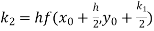
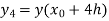
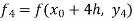
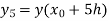
Solution of Second order ODE using 4th order Runge-Kutta method:
The second order differential equation
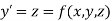
Let
Then |


This can be solved as we discuss above by RungeKutta Method. Here  for
for  and
and  for
for  .
.
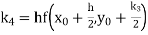
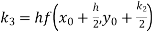
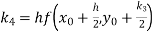
A fourth order Runge Kutta formula:
Where
|


Example1: Using Runge Kutta method of order four,
solve |

Given second order differential equation is
Let Or
Or By RungeKutta Method we have
A fourth order Runge Kutta formula:
|


Example2: Using RungeKutta method, solve
 for
for correct to four decimal places with initial condition
  .
.
Given second order differential equation is
Let Or
Or By Runge-Kutta Method we have
A fourth order Runge Kutta formula:
And
|
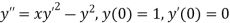


Example3: Solve the differential equations
|
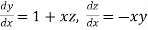

Using four order RungeKutta method with initial conditions 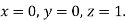
Given differential equation are
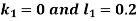
Let
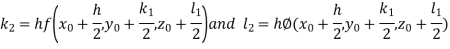
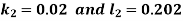
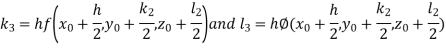
And Also By RungeKutta Method we have
A fourth order Runge Kutta formula:
And
|


Key takeaways
Where |


Milne’s predictor corrector formula-
For given dy/dx = f(x,y) and y = |


We follow the steps given below-
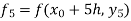
The value  being given, here we calculate-
|

By Taylor’s series or Picard’s method.
Now we calculate-
Then to find We substitute Newton’s forward interpolation formula-
In the relation-
By putting x =
Neglecting fourth and higher order differences and expressing
This is called a predictor. Now having found Then the better value of
Which is called corrector. Then an improved value of We continues this step until Once
And
Then the better approximation to the value of
We repeat until |


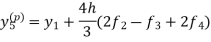

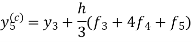


This is called the Milne’s predictor-corrector method.
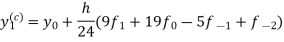
Adams - Bashforth predictor and corrector formula-
This is called Adams - Bashforth predictor formula. And
|
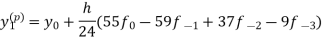

This is called Adams - Bashforth corrector formula.
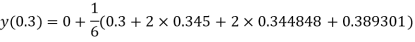
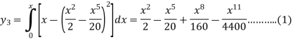
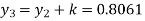
Example: Find the solution of the differential equation  in the range
  for the boundary conditions y = 0 and x = 0 by using Milne’s method.
Sol.
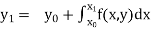
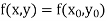
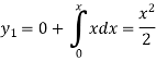
By using Picards method-
Where
To get the first approximation- We put y = 0 in f(x, y), Giving-
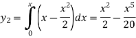
In order to find the second approximation, we put y = Giving-
And the third approximation-
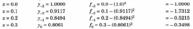
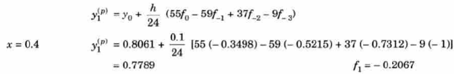
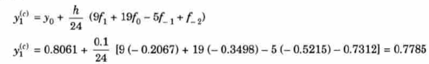
Now determine the starting values of the Milne’s method from equation (1), by choosing h = 0.2
Now using the predictor-
X = 0.8
And the corrector-
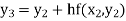
Now again using corrector- Using predictor-
X = 1.0,
And the corrector-
Again using corrector-
Hence
|


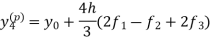


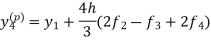


Example: Solve the intital value problem
|

y(0) = 1 to find y(0.4) by using Adams-Bashforth method.
Starting solutions required are to be obtained using Runge-Kutta method of order 4 using step value h = 0.1
Sol.
Here we have-
Here So that-
Thus
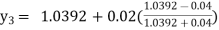
To find y(0.2)- Here
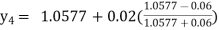
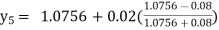
Thus, Y(0.2) = To find y(0.3)- Here
Thus, Y(0.3) = Now the starting values of Adam’s method with h = 0.1-
Using predictor-
Using corrector-
Hence
|


Key takeaways
|


References
- E. Kreyszig, “Advanced Engineering Mathematics”, John Wiley & Sons, 2006.
- P. G. Hoel, S. C. Port And C. J. Stone, “Introduction To Probability Theory”, Universal Book Stall, 2003.
- S. Ross, “A First Course in Probability”, Pearson Education India, 2002.
- W. Feller, “An Introduction To Probability Theory and Its Applications”, Vol. 1, Wiley, 1968.
- N.P. Bali and M. Goyal, “A Text Book of Engineering Mathematics”, Laxmi Publications, 2010.
- B.S. Grewal, “Higher Engineering Mathematics”, Khanna Publishers, 2000.
- T. Veerarajan, “Engineering Mathematics”, Tata Mcgraw-Hill, New Delhi, 2010
- Higher engineering mathematics, HK Dass


