Unit 6
Random variables
It is a real valued function which assigns a real number to each sample point in the sample space.
A random variable X is a function defined on the sample space 5 of an experiment S of an experiment. Its value are real numbers. For every number a the probability
With which X assumes a is defined. Similarly for any interval l the probability
With which X assumes any value in I is defined. |


Example:
Tossing a fair coin thrice then-
Sample Space(S) = {HHH, HHT, HTH, THH, HTT, THT, TTH, TTT}
2. Roll a dice Sample Space(S) = {1,2,3,4,5,6} |
A random variable is a real-valued function whose domain is a set of possible outcomes of a random experiment and range is a sub-set of the set of real numbers and has the following properties:
i) Each particular value of the random variable can be assigned some probability
ii) Uniting all the probabilities associated with all the different values of the random variable gives the value 1.
A random variable is denoted by X, Y, Z etc.
For example if a random experiment E consists of tossing a pair of dice, the sum X of the two numbers which turn up have the value 2,3,4,…12 depending on chance. Then X is a random variable
Discrete random variable-
A random variable is said to be discrete if it has either a finite or a countable number of values. Countable number of values means the values which can be arranged in a sequence.
Note- if a random variable takes a finite set of values it is called discrete and if if a random variable takes an infinite number of uncountable values it is called continuous variable.
Discrete probability distributions-
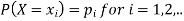
Let X be a discrete variate which is the outcome of some experiments. If the probability that X takes the values of x is  , then-
Where- 1. 2. |

The set of values  with their probabilities
  makes a discrete probability distribution of the discrete random variable X.
Probability distribution of a random variable X can be exhibited as follows-
X |
|
|
|
P(x) |
|
|
|


Example: Find the probability distribution of the number of heads when three coins are tossed simultaneously.
Sol.
Let be the number of heads in the toss of three coins
The sample space will be- {HHH, HHT, HTH, THH, HTT, THT, TTH, TTT} Here variable X can take the values 0, 1, 2, 3 with the following probabilities- P[X= 0] = P[TTT] = 1/8 P[X = 1] = P [HTT, THH, TTH] = 3/8 P[X = 2] = P[HHT, HTH, THH] = 3/8 P[X = 3] = P[HHH] = 1/8 |
Hence the probability distribution of X will be-
X |
|
|
|
|
P(x) |
|
|
|
|


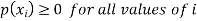
Example: For the following probability distribution of a discrete random variable X,
Find-
1. The value of c.
2. P[1<x<4]
Sol,
1. We know that-
So that- 0 + c + c + 2c + 3c + c = 1 8c = 1 Then c = 1/8 Now, 2. P[1<x<4] = P[X = 2] + P[X = 3] = c + 2c = 3c = 3× 1/8 = 3/8
|

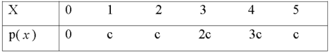
Probability density function (PDF) is a arithmetical appearance which gives a probability distribution for a discrete random variable as opposite to a continuous random variable. The difference among a discrete random variable is that we check an exact value of the variable. Like, the value for the variable, a stock worth, only goes two decimal points outside the decimal (Example 32.22), while a continuous variable have an countless number of values (Example 32.22564879…).
When the PDF is graphically characterized, the area under the curve will show the interval in which the variable will decline. The total area in this interval of the graph equals the probability of a discrete random variable happening. More exactly, since the absolute prospect of a continuous random variable taking on any exact value is zero owing to the endless set of possible values existing, the value of a PDF can be used to determine the likelihood of a random variable dropping within a exact range of values.
|
Example: The probability density function of a variable X is
X | 0 | 1 | 2 | 3 | 4 | 5 | 6 |
P(X) | k | 3k | 5k | 7k | 9k | 11k | 13k |
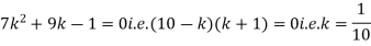
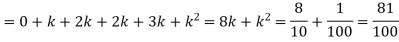
(i) Find (ii) What will be e minimum value of k so that |


Solution
i) If X is a random variable then
Thus, minimum value of k=1/30. |

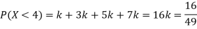
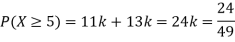
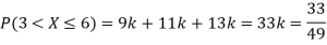
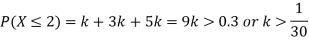
Example: A random variate X has the following probability function
x | 0 | 1 | 2 | 3 | 4 | 5 | 6 | 7 |
P (x) | 0 | k | 2k | 2k | 3k |
|
|
|


(i) Find the value of the k. (ii) |

Solution.
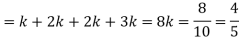
(i) If X is a random variable then
|


Continuous probability distribution
When a variate X takes every value in an interval it gives rise to continuous distribution of X. The distribution defined by the vidiots like heights or weights are continuous distributions.
a major conceptual difference however exist between discrete and continuous probabilities. When thinking in discrete terms the probability associated with an event is meaningful. With continuous events however where the number of events is infinitely large, the probability that a specific event will occur is practically zero. for this reason, continuous probability statements on must be worth did some work differently from discrete ones. Instead of finding the probability that x equals some value, we find the probability of x falling in a small interval.
Thus the probability distribution of a continuous variate x is defined by a function f (x) such that the probability of the variate x falling in the small interval |
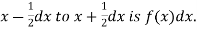
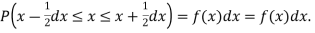
The range of the variable may be finite or infinite. But even when the range is finite, it is convenient to consider it as infinite by opposing the density function to be zero outside the given range. Thus if f (x) =(x) be the density function denoted for the variate x in the interval (a,b), then it can be written as
|
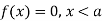

The density function f (x) is always positive and 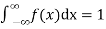 (i.e. the total area under the probability curve and the the x-axis is is unity which corresponds to the requirements that the total probability of happening of an event is unity).
(2) Distribution function
If |
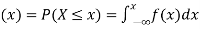
Then F(x) is defined as the commutative distribution function or simply the distribution function the continuous variate X. It is the probability that the value of the variate X will be ≤x. The graph of F(x) in this case is as shown in figure 26.3 (b).
The distribution function F (x) has the following properties
(i) (ii) (iii) (iv) P(a ≤x ≤b)= |


Example.
(i) Is the function defined as follows a density function.
(ii) If so determine the probability that the variate having this density will fall in the interval (1.2). (iii) Also find the cumulative probability function F (2)? |

Solution.
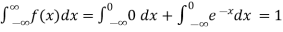
(i) f (x) is clearly ≥0 for every x in (1,2) and
Hence the function f (x) satisfies the requirements for a density function. (ii)Required probability = This probability is equal to the shaded area in figure 26.3 (a). (iii)Cumulative probability function F(2)
Which is shown in figure |


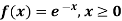
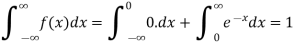
Example: Show that the following function can be defined as a density function and then find  .
.
|
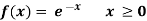

Sol.
here
So that, the function can be defined as a density function. Now.
|
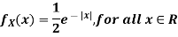
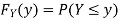
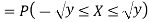
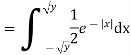
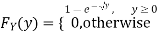
Example: Let X be a continuous random variable with PDF given by
|
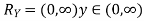
If  , find the CDF of Y.
Solution.
First, we note that
Thus, |


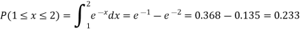
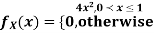
Example: Let X be a continuous random variable with PDF
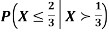
Find |
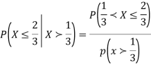
Solution.
We have
|


Key takeaways
1. A random variable is said to be discrete if it has either a finite or a countable number of values. Countable number of values means the values which can be arranged in a sequence. 2. Where- 1. |


BINOMIAL DISTRIBUTION
|
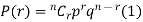
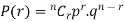
To find the probability of the happening of an event once, twice, thrice,…r times ….exactly in n trails.
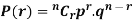
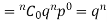
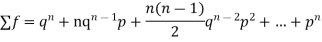
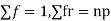
Let the probability of the happening of an event A in one trial be p and its probability of not happening be 1 – p – q. We assume that there are n trials and the happening of the event A is r times and its not happening is n – r times. This may be shown as follows AA……A r times n – r times (1) A indicates its happening We see that (1) has the probability pp…p qq….q= r times n-r times (2) Clearly (1) is merely one order of arranging r A’S. The probability of (1) = The number of different arrangements of r A’s and (n-r) Probability of the happening of an event r times =
If r = 0, probability of happening of an event 0 times If r = 1,probability of happening of an event 1 times If r = 2,probability of happening of an event 2 times If r = 3,probability of happening of an event 3 times These terms are clearly the successive terms in the expansion of Hence it is called Binomial Distribution |


Example. If on an average one ship in every ten is wrecked. Find the probability that out of 5 ships expected to arrive, 4 at least we will arrive safely.
Solution:
Out of 10 ships one ship is wrecked. I.e., nine ships out of 10 ships are safe, P (safety) = P (at least 4 ships out of 5 are safe) = P (4 or 5) = P (4) + P(5)
|


Example. The overall percentage of failures in a certain examination is 20. if 6 candidates appear in the examination what is the probability that at least five pass the examination?
Solution:
Probability of failures = 20% Probability of (P) = Probability of at least 5 pass = P(5 or 6)
|


Example:
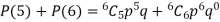
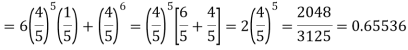
The probability that a man aged 60 will live to be 70 is 0.65. what is the probability that out of 10 men, now 60, at least seven will live to be 70?
Solution:
The probability that a man aged 60 will live to be 70
Number of men= n = 10 Probability that at least 7 men will live to 70 = (7 or 8 or 9 or 10) = P (7)+ P(8)+ P(9) + P(10) =
|


Example
Assuming that 20% of the population of a city are literate so that the chance of an individual being literate is  and assuming that hundred investigators each take 10 individuals to see whether they are illiterate, how many investigators would you expect to report 3 or less were literate.
Solution
Required number of investigators = 0.879126118× 100 =87.9126118 = 88 approximate |


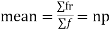
Mean or binomial distribution
|

Successors r | Frequency f | rf |
0 |
| 0 |
1 |
|
|
2 |
| n(n-1) |
3 |
|
|
….. | …… | …. |
n |
|
|


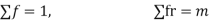
Since, |


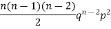
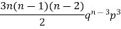
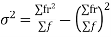
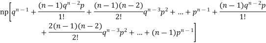
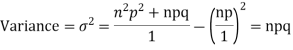
STANDARD DEVIATION OF BINOMIAL DISTRIBUTION
Successors r | Frequency f |
|
0 |
| 0 |
1 |
|
|
2 |
| 2n(n-1) |
3 |
|
|
….. | …… | …. |
n |
|
|


We know that r is the deviation of items (successes) from 0.
Putting these values in (1) we have
Hence for the binomial distribution, Mean |


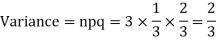
Example. A die is tossed thrice. A success is getting 1 or 6 on a TOSS. Find the mean and variance of the number of successes.
Solution.
|
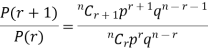
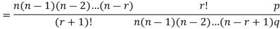
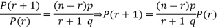
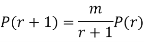
RECURRENCE RELATION FOR THE BINOMIAL DISTRIBUTION
By Binomial Distribution
On dividing (2) by (1) , we get
|

Poisson Distribution:
Poisson distribution is a particular limiting form of the Binomial distribution when p (or q) is very small and n is large enough.
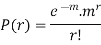
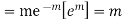
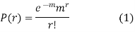
Poisson distribution is
where m is the mean of the distribution. |

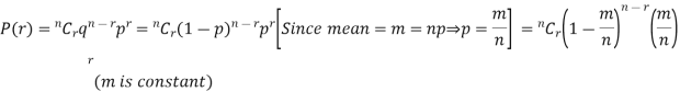
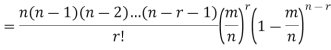
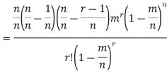
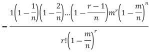
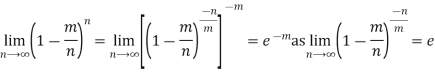
Proof. In Binomial Distribution
Taking limits when n tends to infinity
|


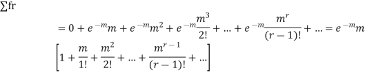
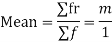
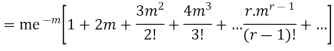
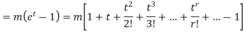
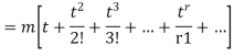
MEAN OF POISSON DISTRIBUTION
|
Success r | Frequency f | f.r |
0 |
| 0 |
1 |
|
|
2 |
|
|
3 |
|
|
… | … | … |
r |
|
|
… | … | … |


|
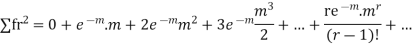
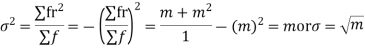
STANDARD DEVIATION OF POISSON DISTRIBUTION
|

Successive r | Frequency f | Product rf | Product |
0 |
| 0 | 0 |
1 |
|
|
|
2 |
|
|
|
3 |
|
|
|
……. | …….. | …….. | …….. |
r |
|
|
|
…….. | ……. | …….. | ……. |


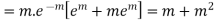
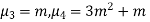
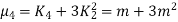
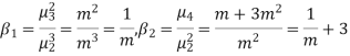
Hence mean and variance of a Poisson distribution are equal to m. Similarly we can obtain,
|


MEAN DEVIATION
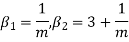
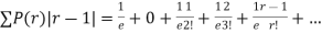
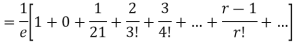
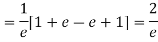
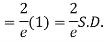
Show that in a Poisson distribution with unit mean, and the mean deviation about the mean is 2/e times the standard deviation.
Solution
|


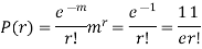
r | P (r) | |r-1| | P(r)|r-1| |
0 |
| 1 |
|
1 |
| 0 | 0 |
2 |
| 1 |
|
3 |
| 2 |
|
4 |
| 3 |
|
….. | ….. | ….. | ….. |
r |
| r-1 |
|


Mean Deviation =
|


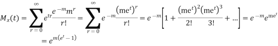
MOMENT GENERATING FUNCTION OF POISSON DISTRIBUTION
Solution
Let
|


CUMULANTS
The cumulant generating function
Now i.e. Mean =
|


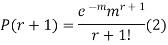
RECURRENCE FORMULA FOR POISSON DISTRIBUTION
SOLUTION.
By Poisson distribution
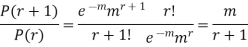
On dividing (2) by (1) we get
|

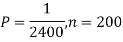
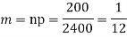
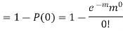
Example. Assume that the probability of an individual coal miner being killed in a mine accident during a year is  . Use appropriate statistical distribution to calculate the probability that in a mine employing 200 miners, there will be at least one fatal accident in a year.
Solution
|


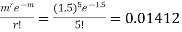
Example. Suppose 3% of bolts made by a machine are defective, the defects occuring at random during production. If bolts are packaged 50 per box, find
(a) Exact probability and
(b) Poisson approximation to it, that a given box will contain 5 defectives.
Solution
(a) Hence the probability for 5 defectives bolts in a lot of 50.
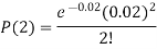
(b) To get Poisson approximation m = np = Required Poisson approximation= |

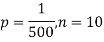
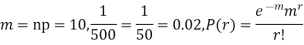
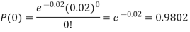
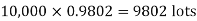
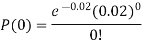
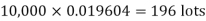
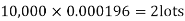
Example. In a certain factory producing cycle tyres, there is a smallchance of 1 in 500 tyres to be defective. The tyres are supplied in lots of 10. Using Poisson distribution, calculate the approximate number of lots containing no defective, one defective and two defective tyres, respectively, in a consignment of 10,000 lots.
Solution.
|
S.No. | Probability of defective | Number of lots containing defective |
1. |
|
|
2. |
|
|
3. |
|
|

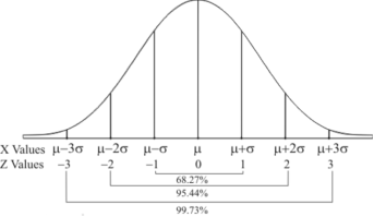
Normal Distribution-
The concept of normal distribution was given by English mathematician Abraham De Moivre in 1733 but the concrete theory was given by Karl Gauss that is why sometime normal distribution is called Gaussian distribution.
Normal distribution is a continuous distribution. It is a limiting case of binomial distribution.
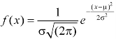
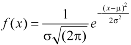
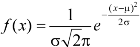
The probability density function of a normal distribution is given by-
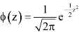
Here Where Note- 1. If a random variable X follows normal distribution with mean 2. If X 3. The probability density function of standard normal variate Z is given as-
Where |


Graph of a normal probability function-
The curve look like bell-shaped curve. The top of the bell is exactly above the mean.
If the value of standard deviation is large then curve tends to flatten out and for small standard deviation it has sharp peak.
This is one of the most important probability distributions in statistical analysis.
|
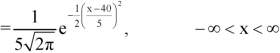
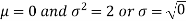
Example:
1. If X  then find the probability density function of X.
2. If X  then find the probability density function of X.
Sol.
1. We are given X Here We know that-
Then the p.d.f. will be-
2. . We are given X Here We know that-
Then the p.d.f. will be-
|


Mean, median and mode of the normal distribution-
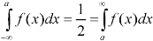
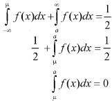
Let ‘a’ is the median, then it divides the total area into two parts-
Where-
Let a>mean, then-
Thus-
So that mean = median.
Note- mean deviation about mean is = |


Mode-
The mode of the normal distribution is
Hence the mean, median and mode are equal in normal distribution |


.
Area property of a normal distribution (Area under the normal curve)-
Let X follows the normal distribution with mean We form a normal curve by taking Note- Total area under the curve is always 1. |


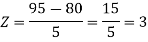
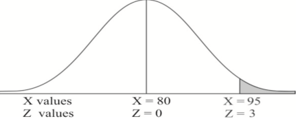
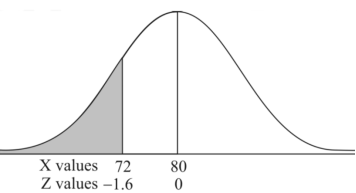
Example: If a random variable X is normally distributed with mean 80 and standard deviation 5, then find-
1. P[X > 95]
2. P[X < 72]
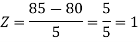
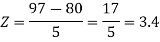
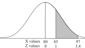
3. P [85 < X <97]
[Note- use the table- area under the normal curve]
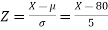
Sol.
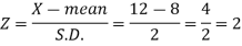
The standard normal variate is – Now- 1. X = 95,
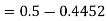
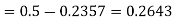
So that-
2. X = 72,
So that-
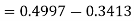
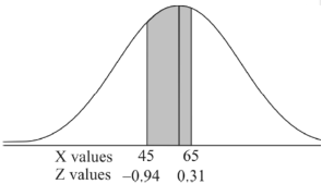
3. X = 85,
X = 97,
So that-
|


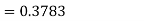
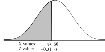
Example: In a company the mean weight of 1000 employees is 60kg and standard deviation is 16kg.
Find the number of employees having their weights-
1. Less than 55kg.
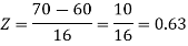
2. More than 70kg.
3. Between 45kg and 65kg.
Sol.
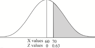
Suppose X be a normal variate = the weight of employees. Here mean 60kg and S.D. = 16kg X Then we know that-
We get from the data,
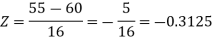
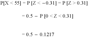
Now- 1. For X = 55,
So that-
2. For X = 70,
So that-
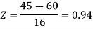
3. For X = 45,
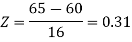
For X = 65,
Hence the number of employees having weights between 45kg and 65kg-
|


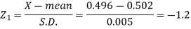
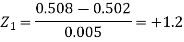
Example: The mean inside diameter of a sample of 200 washers produced by a machine is 0.0502 cm and the standard deviation is 0.005 cm. The purpose for which these washers are intended allows a maximum tolerance in the diameter of 0.496 to 0.508 cm, otherwise the washers are considered defective. Determine the percentage of defective washers produced by the machine, assuming the diameters are normally distributed.
Sol.
Here-
And
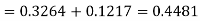
Area for non-defective washers = area between z = -1.2 to +1.2 = 2 area between z = 0 and z = 1.2 = 2 × 0.3849 = 0.7698 = 76.98% Then percent of defective washers = 100 – 76.98 = 23.02 % |
Example: The life of electric bulbs is normally distributed with mean 8 months and standard deviation 2 months.
If 5000 electric bulbs are issued how many bulbs should be expected to need replacement after 12 months?
[Given that P (z ≥ 2) = 0. 0228]
Sol.
Here mean (μ) = 8 and standard deviation = 2 Number of bulbs = 5000 Total months (X) = 12 We know that-
Area (z ≥ 2) = 0.0228 Number of electric bulbs whose life is more than 12 months ( Z> 12) = 5000 × 0.0228 = 114 Therefore replacement after 12 months = 5000 – 114 = 4886 electric bulbs.
|
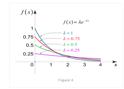
The exponential distribution is a C.D. which is usually use to define to come time till some precise event happens. Like, the amount of time until a storm or other unsafe weather event occurs follows an exponential distribution law.
The one-parameter exponential distribution of the probability density function PDF is defined:
f(x)=λ
Where, the rate λ signifies the Normal amount of events in single time.
|

The mean value is μ =  . The median of the exponential distribution is m =
  , and the variance is shown by
  .
.
Key takeaways
3. MOMENT GENERATING FUNCTION OF POISSON DISTRIBUTION
4. RECURRENCE FORMULA FOR POISSON DISTRIBUTION
5. Normal Distribution- The probability density function of a normal distribution is given by-
Here
|


References
- E. Kreyszig, “Advanced Engineering Mathematics”, John Wiley & Sons, 2006.
- P. G. Hoel, S. C. Port And C. J. Stone, “Introduction To Probability Theory”, Universal Book Stall, 2003.
- S. Ross, “A First Course in Probability”, Pearson Education India, 2002.
- W. Feller, “An Introduction To Probability Theory and Its Applications”, Vol. 1, Wiley, 1968.
- N.P. Bali and M. Goyal, “A Text Book of Engineering Mathematics”, Laxmi Publications, 2010.
- B.S. Grewal, “Higher Engineering Mathematics”, Khanna Publishers, 2000.
- T. Veerarajan, “Engineering Mathematics”, Tata Mcgraw-Hill, New Delhi, 2010
- Higher engineering mathematics, HK Dass


