Unit 8
Concept of joint probability
Let X and Y be two discrete random variables defined on the sample space S of a random experiment then the function (X, Y) defined on the same sample space is called a two-dimensional discrete random variable. In others words, (X, Y) is a two-dimensional random variable if the possible values of (X, Y) are finite or countably infinite. Here, each value of X and Y is represented as a point ( x, y ) in the xy-plane.
Joint probability mass function-
Let (X, Y) be a two-dimensional discrete random variable. With each possible
Outcome ( we associate a number p(
 representing
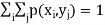
Where P [X =  satisfies the following conditions-
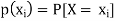
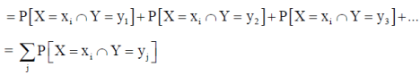
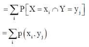
The function ‘p’ is called joint probability mass function of X and Y. if (X, Y) is a discrete two-dimensional random variable which take up the values (
which is known as the marginal probability mass function of X. Similarly, the probability distribution of Y is
and is known as the marginal probability mass function of Y. |


Conditional Probability Mass Function-
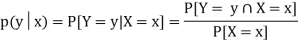
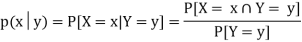
Let (X, Y) be a discrete two-dimensional random variable. Then the conditional probability mass function of X, given Y y is defined as
The conditional probability mass function of Y, given X = x, is defined as
|

Independence of random variables-
Two discrete random variables X and Y are said to be independent iff-
|

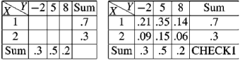
Example: Find the joint distribution of X and
Y , which are independent random variables with the
following respective distributions:
| 1 | 2 |
P [ X = | 0.7 | 0.3 |


And
| -2 | 5 | 8 |
P [ Y = | 0.3 | 0.5 | 0.2 |


Sol.
Since X and Y are independent random variables,
Thus, the entries of the joint distribution are the products of the marginal entries
|

Example: The following table represents the joint probability distribution of
the discrete random variable (X, Y):
X/Y | 1 | 2 |
1 | 0.1 | 0.2 |
2 | 0.1 | 0.3 |
3 | 0.2 | 0.1 |
Then find-
i) The marginal distributions. ii) The conditional distribution of X given Y = 1. iii) P[(X + Y) < 4]. |
Sol.
i) The marginal distributions.
X/Y | 1 | 2 | p(x) [totals] |
1 | 0.1 | 0.2 | 0.3 |
2 | 0.1 | 0.3 | 0.4 |
3 | 0.2 | 0.1 | 0.3 |
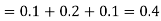
p(y) [ totals] | 0.4 | 0.6 | 1 |
The marginal probability distribution of X is-
X | 1 | 2 | 3 |
p(x) | 0.3 | 0.4 | 0.3 |
The marginal probability distribution of Y is
Y | 1 | 2 |
p(x) | 0.4 | 0.6 |
ii) The conditional distribution of X given Y = 1.
|
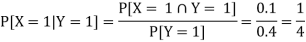
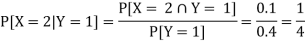
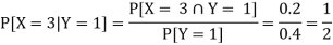
The conditional distribution of X given Y = 1 is-
X | 1 | 2 | 3 |
| ¼ | 1/4 | ½ |

(iii) The values of (X, Y) which satisfy X + Y < 4 are (1, 1), (1, 2) and (2, 1)
only.
Which gives-
|

Example: Find-
(a) Marginal distributions
(b) E(X) and E(Y )
(c) Cov (X, Y )
(d) σX , σY and
(e) ρ(X, Y )
For the following joint probability distribution-
|
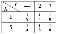
Sol.
(a) Marginal distributions
|
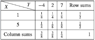
The marginal distribution of x
X | 1 | 5 |
p(x) | 1/2 | 1/2 |
The marginal distribution of Y-
Y | -4 | 2 | 7 |
p(y) | 3/8 | 3/8 | ¼ |
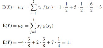
(b) E(X) and E(Y )
|
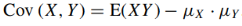
(c) Cov (X, Y )
As we know that-
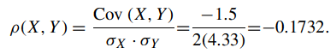
= -1.5 |
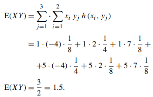

(d) σX , σY and
|
(e) ρ(X, Y )
|
Key takeaways
2. Independence of random variables- Two discrete random variables X and Y are said to be independent iff-
|

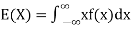
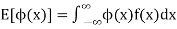
Expectation
The mean value of the probability distribution of a variate X is commonly known as its expectation current is denoted by E (X). If f(x) is the probability density function of the variate X, then
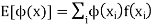
In general expectation of any function is
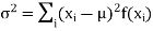
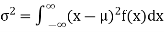
(2) Variance offer distribution is given by
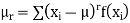
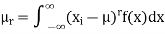
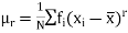
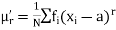
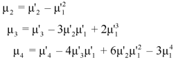
Where (3) The rth moment about mean (denoted by
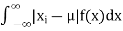
(4) Mean deviation from the mean is given by
|


Example. In a lottery, m tickets are drawn at a time out of a ticket numbered from 1 to n. Find the expected value of the sum of the numbers on the tickets drawn.
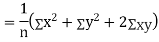
Solution. Let  be the variables representing the numbers on the first, second, nth ticket. The probability of drawing a ticket out of n ticket spelling in each case 1/n, we have
|
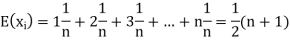
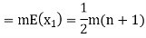
Therefore, expected value of the sum of the numbers on the tickets drawn
|

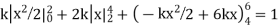
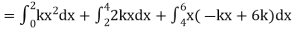
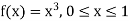
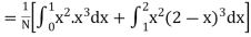
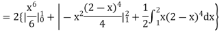
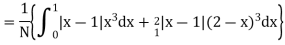
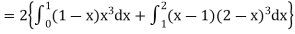
Example. X is a continuous random variable with probability density function given by
|
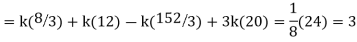
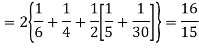
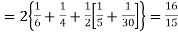
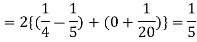
Find k and mean value of X.
Solution.
Since the total probability is unity.
Mean of X =
|


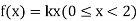
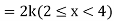
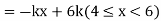
Example. The frequency distribution of a measurable characteristic varying between 0 and 2 is as under
|
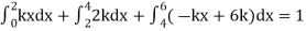
Calculate two standard deviation and also the mean deviation about the mean.
Solution.
Total frequency N =
Hence, i.e., standard deviation Mean derivation about the mean
|


Variance of a sum
One of the applications of covariance is finding the variance of a sum of several random variables. In particular, if Z = X + Y, then
Var (Z) =Cov (Z,Z)
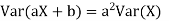
More generally, for a, b
|


Variance
Consider two random variables X and Y with the following PMFs
|
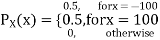
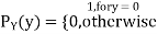
Note that EX =EY = 0. Although both random variables have the same mean value, their distribution is completely different. Y is always equal to its mean of 0, while X is IDA 100 or -100, quite far from its mean value. The variance is a measure of how spread out the distribution of a random variable is. Here the variance of Y is quite small since its distribution is concentrated value. Why the variance of X will be larger since its distribution is more spread out.
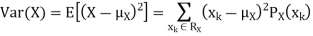
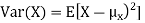
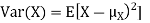
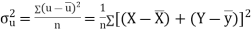
The variance of a random variable X with mean  , is defined as
|
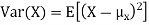
By definition the variance of X is the average value of  Since
Since  ≥0, the variance is always larger than or equal to zero. A large value of the variance means that
  is often large, so X often X value far from its mean. This means that the distribution is very spread out. on the other hand a low variance means that the distribution is concentrated around its average.
Note that if we did not square the difference between X and its mean the result would be zero. That is
|

X is sometimes below its average and sometimes above its average. Thus  is sometimes negative and sometimes positive but on average it is zero.
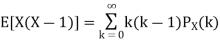
To compute
For example, for X and Y defined in equations 3.3 and 3.4 we have
As we expect, X has a very large variance while Var (Y) = 0 |


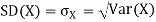
Note that Var (X) has a different unit than X. For example, if X is measured in metres then Var(X) is in  .to solve this issue we define another measure called the standard deviation usually shown as
  which is simply the square root of variance.
The standard deviation of a random variable X is defined as
The standard deviation of X has the same unit as X. For X and Y defined in equations 3.3 and 3.4 we have
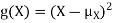
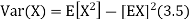
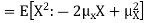
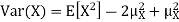
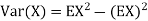
Here is a useful formula for computing the variance. Computational formula for the variance
To prove it note that
Note that for a given random variable X,
Equation 3.5 is equally easier to work with compared to
And then subtract |


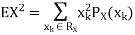

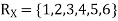
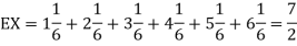
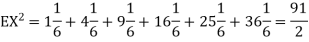
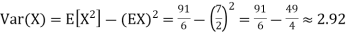
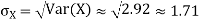
Example. I roll a fair die and let X be the resulting number. Find E(X), Var(X), and 
Solution.
We have
Thus ,
|

Theorem
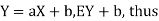
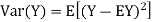
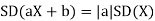
For random variable X and real number, a and b
|

Proof.
If
From equation 3.6, we conclude that, for standard deviation, |

Theorem
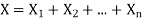
If  are independent random variables and
  , then
|

Example. If  Binomial (n, p) find Var (X).
Solution.
We know that we can write a Binomial (n, p) random variable as the sum of n independent Bernoulli (p) random variable, i.e.
If
|


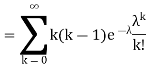
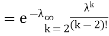
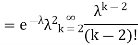
Problem. If  , find Var (X).
Solution.
We already know
S
So we have
|


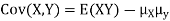
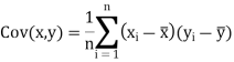
Covariance-
We denote the covariance of X and Y by Cov(x, y) and it is given as-
|
Correlation coefficient
Whenever two variables x and y are so related that an increase in the one is accompanied by an increase or decrease in the other, then the variables are said to be correlated.
For example, the yield of crop varies with the amount of rainfall.
If an increase in one variable corresponds to an increase in the other, the correlation is said to be positive. If increase in one corresponds to the decrease in the other the correlation is said to be negative. If there is no relationship between the two variables, they are said to be independent.
Perfect Correlation:
If two variables vary in such a way that their ratio is always constant, then the correlation is said to be perfect.
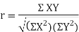
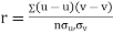
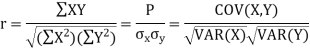
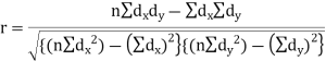
KARL PEARSON’S COEFFICIENT OF CORRELATION:
Here-
|


Note-
1. Correlation coefficient always lies between -1 and +1.
2. Correlation coefficient is independent of change of origin and scale.
3. If the two variables are independent then correlation coefficient between them is zero.
Correlation coefficient | Type of correlation |
+1 | Perfect positive correlation |
-1 | Perfect negative correlation |
0.25 | Weak positive correlation |
0.75 | Strong positive correlation |
-0.25 | Weak negative correlation |
-0.75 | Strong negative correlation |
0 | No correlation |
Example: Find the correlation coefficient between Age and weight of the following data-
Age | 30 | 44 | 45 | 43 | 34 | 44 |
Weight | 56 | 55 | 60 | 64 | 62 | 63 |
Sol.
x | y |
|
|
|
| ( |
30 | 56 | -10 | 100 | -4 | 16 | 40 |
44 | 55 | 4 | 16 | -5 | 25 | -20 |
45 | 60 | 5 | 25 | 0 | 0 | 0 |
43 | 64 | 3 | 9 | 4 | 16 | 12 |
34 | 62 | -6 | 36 | 2 | 4 | -12 |
44 | 63 | 4 | 16 | 3 | 9 | 12 |
Sum= 240 |
360 |
0 |
202 |
0 |
70
|
32 |


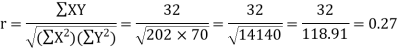
Karl Pearson’s coefficient of correlation-
Here the correlation coefficient is 0.27. which is the positive correlation (weak positive correlation), this indicates that the as age increases, the weight also increase. |
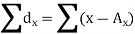
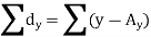
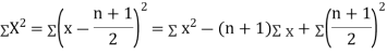
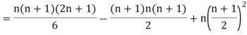
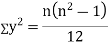
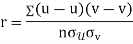
Short-cut method to calculate correlation coefficient-
Here,
|

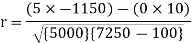
Example: Find the correlation coefficient between the values X and Y of the dataset given below by using short-cut method-
X | 10 | 20 | 30 | 40 | 50 |
Y | 90 | 85 | 80 | 60 | 45 |
Sol.
X | Y |
|
|
|
|
|
10 | 90 | -20 | 400 | 20 | 400 | -400 |
20 | 85 | -10 | 100 | 15 | 225 | -150 |
30 | 80 | 0 | 0 | 10 | 100 | 0 |
40 | 60 | 10 | 100 | -10 | 100 | -100 |
50 | 45 | 20 | 400 | -25 | 625 | -500 |
Sum = 150 |
360 |
0 |
1000 |
10 |
1450 |
-1150 |


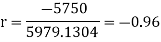
Short-cut method to calculate correlation coefficient-
|

Example: Ten students got the following percentage of marks in Economics and Statistics
Calculate the 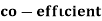 of correlation.
Roll No. |
|
|
|
|
|
|
|
|
|
|
Marks in Economics |
|
|
|
|
|
|
|
|
|
|
Marks in |
|
|
|
|
|
|
|
|
|
|


Solution:
Let the marks oftwo subjects be denoted by  and
and  respectively.
Then the mean for  marks
marks  and the mean ofy marks
 and
and are deviations ofx’s and
  ’s from their respective means, then the data may be arranged in the following form:
x | y | X=x=65 | Y=y=66 |
|
| XY |
78 | 84 | 13 | 18 | 169 | 234 | 234 |
36 | 51 | -29 | -15 | 841 | 225 | 435 |
98 | 91 | 33 | 1089 | 1089 | 625 | 825 |
25 | 60 | -40 | 1600 | 1600 | 36 | 240 |
75 | 68 | 10 | 100 | 100 | 4 | 20 |
82 | 62 | 17 | 289 | 289 | 16 | -68 |
90 | 86 | 25 | 625 | 625 | 400 | 500 |
62 | 58 | -3 | 9 | 9 | 64 | 24 |
65 | 53 | 0 | 0 | 0 | 169 | 0 |
39 | 47 | -26 | 676 | 676 | 361 | 494 |
650 | 660 | 0 | 5398 | 5398 | 2224 | 2704 |


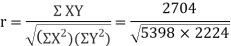
Here,
|

Spearman’s Rank Correlation
|
Solution:
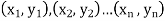
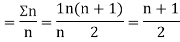
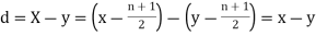
Let Assuming nor two individuals are equal in either classification, each individual takes the values 1, 2, 3,
Let Then where
Clearly,
|


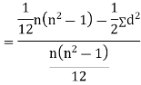
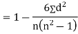
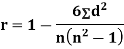
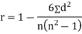
SPEARMAN’S RANK CORRELATION COEFFICIENT:
|

Where  denotes the rank coefficient of correlation and
  refers to the difference ofranks between paired items in two series.
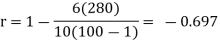
Example: Compute Spearman’s rank correlation coefficient r for the following data:
Person | A | B | C | D | E | F | G | H | I | J |
Rank Statistics | 9 | 10 | 6 | 5 | 7 | 2 | 4 | 8 | 1 | 3 |
Rank in income | 1 | 2 | 3 | 4 | 5 | 6 | 7 | 8 | 9 | 10 |
Solution:
Person | Rank Statistics | Rank in income | d= |
|
A | 9 | 1 | 8 | 64 |
B | 10 | 2 | 8 | 64 |
C | 6 | 3 | 3 | 9 |
D | 5 | 4 | 1 | 1 |
E | 7 | 5 | 2 | 4 |
F | 2 | 6 | -4 | 16 |
G | 4 | 7 | -3 | 9 |
H | 8 | 8 | 0 | 0 |
I | 1 | 9 | -8 | 64 |
J | 3 | 10 | -7 | 49 |


|

Example:
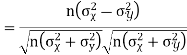
If X and Y are uncorrelated random variables,  the
the  of correlation between
  and
and 
Solution:
Let Then Now Similarly Now
Also
Similarly
|


Key takeaways
2. Correlation coefficient always lies between -1 and +1. 3. Correlation coefficient is independent of change of origin and scale. 4. If the two variables are independent then correlation coefficient between them is zero. 5. Short-cut method to calculate correlation coefficient-
6. Spearman’s Rank Correlation
4. 5. For random variable X and real number a and b
6. If
|


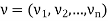
Probability vector-
Probability vector is a vector-
If |


Stochastic process-
Stochastic process is a family of random variables {X(t )|t ∈ T } defined on a common sample space S and indexed by the parameter t , which varies on an index set T .
The values assumed by the random variables X(t ) are called states, and the set of all possible values from the state space of the process is denoted by I .
If the state space is discrete, the stochastic process is known as a chain.
A stochastic process consists of a sequence of experiments in which each experiment has a finite number of outcomes with given probabilities.
Stochastic matrices-
All the entries of square matrix P are non-negative and the sum of the entries of any row is one.
A vector v is said to be a fixed vector or a fixed point of a matrix A if vA = v and v = 0. if v is a fixed vector of A, so is kv since (kv)A = k(vA) = k(v) = kv. |
Note-
3. The transition matrix P of a Markov chain is a stochastic matrix. |


Example: Which vectors are probability vectors?
- (5/2, 0, 8/3, 1/6, 1/6)
- (3, 0, 2, 5, 3)
Sol.
- It is not a probability vector because the sum of the components do not add up to 1
- Dividing by 3 + 0 + 2 + 5 + 3 = 13, we get the probability vector
(3/13, 0, 2/13, 5/13, 3/13)
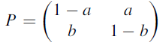
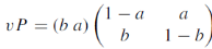
Example: show that
Sol.
|


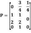
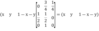
Example: Find the unique fixed probability vector t of
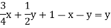
Sol. Suppose t = (x, y, z) be the fixed probability vector. By definition x + y + z = 1. So t = (x, y, 1 − x − y), t is said to be fixed vector, if t P = t
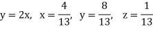
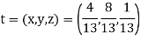
On solving, we get-
Required fixed probability vector is-
|


Markov chain-
Markov chain is a finite stochastic process consisting
of a sequence of trials whose outcomes say  satisfy the following two conditions:
- Each outcome belongs to the state space I = {
 which is the finite set of outcomes.
 - The outcome of any trial depends at most upon the outcome of the immediately preceding trial and not upon any other previous outcomes.
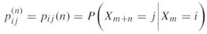
Higher transition probabilities-
The probability that a Markov chain will move from state i to state j in exactly n steps, is denoted by 
And defined as-
|
Stationary distribution-
Stationary distribution of a Markov chain is the unique fixed probability vector t of the regular transition matrix P of the Markov chain because every sequence of probability distribution approach t.
Absorbing States-
A state ai of a Markov chain is said to be an absorbing state if the system remains in the state ai once it enters there, i.e., a state ai is absorbing if pii = 1. Thus once a Markov chain enters such an absorbing state, it is destined there to remain forever. In other words the i’th row in P has 1 at the main diagonal (i, i) position and zeros everywhere else.
References
- E. Kreyszig, “Advanced Engineering Mathematics”, John Wiley & Sons, 2006.
- P. G. Hoel, S. C. Port And C. J. Stone, “Introduction To Probability Theory”, Universal Book Stall, 2003.
- S. Ross, “A First Course in Probability”, Pearson Education India, 2002.
- W. Feller, “An Introduction To Probability Theory and Its Applications”, Vol. 1, Wiley, 1968.
- N.P. Bali and M. Goyal, “A Text Book of Engineering Mathematics”, Laxmi Publications, 2010.
- B.S. Grewal, “Higher Engineering Mathematics”, Khanna Publishers, 2000.
- T. Veerarajan, “Engineering Mathematics”, Tata Mcgraw-Hill, New Delhi, 2010
- Higher engineering mathematics, HK Dass


