UNIT-4
TACHEOMETRY
Tacheometric is a branch of surveying in which horizontal and vertical distances are determined by taking an angular observation with an instrument known as a tachometer. The accuracy attained is such that under favourable conditions error will not exceed 1/100. and if the purpose of a survey does not require accuracy, the method is unexcelled.
Tacheometric survey also can be used for Railways, Roadways, and reservoirs etc. Tacheometric surveying is adopted in rough and difficult terrain where direct levelling and chaining are either not possible or very tedious.
Methods of Tacheometry:
The underlying principle common to different methods of the tachometer is that horizontal distance between an instrument station and a point as well as the elevation of the point relative to the instrument can be determined from angle subtended at the instrument station by a known distance at the point and vertical angle from instrument to the point.
The various tacheometric methods employ principle in different ways and differ one another in methods of observation and reduction, but maybe classified under two heads:
(i) The stadia system.
(ii) The tangential system.
In the stadia system, observation is taken with the stadia wires of the tacheometer and in the tangential system the angles of elevation are measured from instrument station to the points with a theodolite and their tangents are used to determine horizontal of the telescope for necessary but stadia system needs only one and is more commonly used.
The Stadia System of Tacheometry:
In the stadia system of tachometer there are two methods of surveying viz:
(i) Fixed hair method, and
(ii) Moveable hair method.
(i) Fixed Hair Method:
In this method, the distance between the stadia hairs is fixed. When a staff is sighted through the telescope, its certain length is intercepted by stadia hair and from tins value of staff intercept, the distance from the instrument to the staff can be determined. The staff intercept varies with its distance from the instrument. This method is most commonly used in the tachometer.
(ii) Moveable Hair Method:
In these methods, stadia hair are not fixed but can be moved using micrometre screws. The stall is provided with two vanes or targets fixed at a known distance apart. The variable stadia distance is measured, and from this value required horizontal distance may be found out. The method is now rarely used.
Line of sight can be reversed by revolving the telescope by 180* w.r.t. horizontal axis. Transiting is also called as plunging and revering.
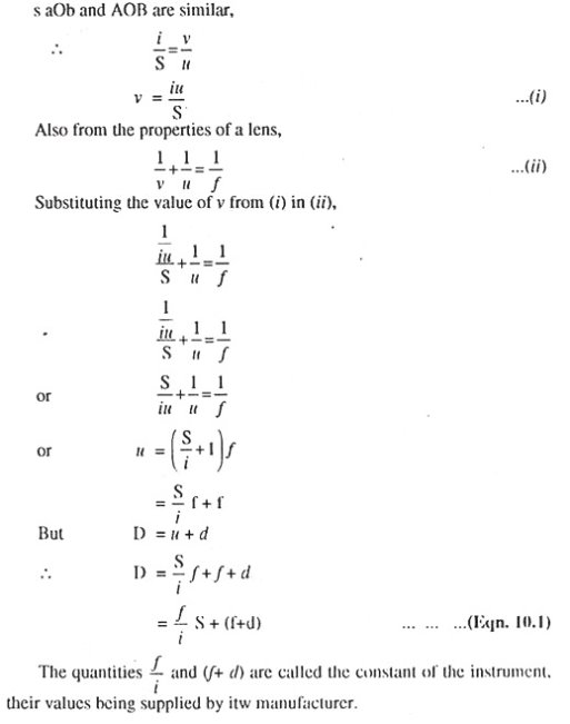
The principle of stadia tachometer is explained as follows: (Fig.)
|

Fig-1 principle of stadia tachometer
Let O= the optical centre of the object-glass
a, b and c= the bottom, top and central hairs at the diagram
A, B and C= the points on the staff cut by three lines a b= I the interval between stadia lines.
(ab is the length of the image of AB)
AB=S=the staff intercept (the differences of the stadia hair readings)
f= the focal length of object-glass i.e, the distance between the centre (O) to the principal focus (FG) of the lens.
u – the horizontal distance from the optical centre (O) to the staff.
v = the horizontal distance from the optical centre (O) to the image of the staff, u and v is called the conjugate focal length of the lens.
d = the horizontal distance from the optical centre (O) to the vertical axis of the tachometer.
D = the horizontal distance from the vertical axis of the instrument to the staff,
Reference 1
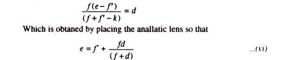
The constant f/i is called the multiple constant and its value is usually 100, while constant (f+d) is called the additive constant and its value varies from 30 cm to 60 cm in case of the external focusing telescope, it is very small varying from 10 cm to 20 cm and is therefore often ignored.
To make the value of additive constant zero, an additional convex lens, known as an analytic lens, is provided in the telescope between the object-glass and eyepiece at a fixed distance from former. By this arrangement, calculation work is reduced considerably.
The equation is applicable only when the line of sight is horizontal and staff is held vertical.
Determination of Stadia Constants of a Tacheometer:
There are two methods available for finding values of the stadia constant f/i and f + d of a given instrument.
First method:
In this method, the values of the constants are obtained by the computations form the field measurements.
Procedure:
(i) Measure accurately a line OA about 300 m long, on fairly level ground and fix pegs along with it at intervals of say, 30m.
(ii) Set up the instrument at O and obtained the staff intercepts by taking stages reading on the staff held vertically at each of pegs.
On substituting the values of D and S in Equations 10.1, we get many equations which when solved in pairs, give several values of the constants:

their mean value is adapted to the values of constants. Thus, if D1, D2, D3, etc.=the distances measured from the instrument, and S1, S2, S3 etc.= the corresponding staff intercepts.
Then we have:
|

Second Method:
In this method, the value of multiplying constant f/i is found by computations from the field measurements and that of additive constant (f+) is obtained by the direct measurements at the telescope.
Procedure:
(i) Sight any far distant – object and focus it.
(ii) Measure accurately the distance along the top of telescope between the object -Glass and the plane of crosshairs (diagram screw) with a rule, the measured distance being equal to focal length (f) of the objective.
(iii) Measure the distance (d) from object— glass to the vertical axis of the instrument.
(iv) Measure several lengths D1, D2, D3 etc. along with OA from the instrument – position O and obtained the staff intercepts S1, S2, S3 ate. at each of these lengths.
(v) Add f and d find values of the additive constant (f+d).
(vi) Knowing (f+d), determined several values of f/i from equation 10. 1.
(vii) The mean of several values gives the required value of multiple constant f/i. Calculation work is much simplified, of the instrument is placed at a distance of (f+d) beyond the beginning O of the line.
Distance and Elevation formulae for Staff Vertical: Inclined Sight
P = Instrument station;
Q = Staff station
M = position of instruments axis;
O = Optical centre of the objective
A, C, B = Points corresponding to the readings of the three hairs
s = AB = Staff intercept;
i = Stadia interval
Ө= Inclination of the line of sight from the horizontal
L= Length MC measured along the line of sight
D= MQ’ = Horizontal distance between the instrument and the staff
V= Vertical intercept at Q, between the line of sight and the horizontal line
h= height of the instrument;
r = central hair reading
β= angle between the two extreme rays corresponding to stadia hairs.
•Draw a line A’CB’ normal to the line of sight OC.
• Angle AAC = 900+ β/2, being the exterior angle of the ∆COA.
•Similarly, from ∆COB, angle OBC = angle BBC = 90o–β/2.
|
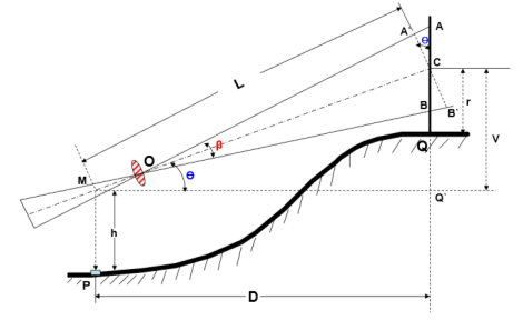
Fig-2 Distance and Elevation formulae for Staff Vertical: Inclined Sight
∟AA’C = ∟BB’C = 900 From ∆ACA’, A’C = AC cos Ө or A’B’ = AB cos Ө = s cos Ө..........(a) Since the line, A’B’ is perpendicular to the line of sight OC, equation D = k s + C is directly applicable. Hence, we have MC = L = k . A’B’ + C = k s cosӨ + C . . . . . . . (b) The horizontal distance D = L cosӨ = (k s cosӨ + C) cosӨ D = k s cos2Ө + C cosӨ. . . . . . (1) Similarly, V = L sin Ө = (k s cosӨ + C) sinӨ = k s cosӨ . sinӨ + C sinӨ V = k s + C sinӨsin2Ө 2 . . . . . . (2) |
Thus above 2 equations are the distance and elevation formulae for the inclined line of sight.
a)Elevation of the staff station for the angle of elevation
If the line of sight has an angle of elevation Ө, as shown in the figure,
Elevation of staff station = Elevation of instrument station + h + V – r.
(b) Elevation of the staff station for the angle of depression:
Elevation of Q = Elevation of P + h – V – r
Distance and Elevation formulae for Staff Normal: Inclined Sight
|
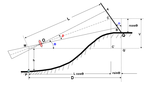
Fig-3 Distance and Elevation formulae for Staff Normal: Inclined Sight
Case (a): Line of Sight at an angle of elevation Ө
Where AB = s = staff intercept;
CQ = r = axial hair reading With the same notations as in the last case,
MC = L = K s + C
The horizontal distance between P and Q is given by
D = MC’ + C’Q’ = L cosӨ + r sinӨ
= (k s + C) cosӨ + r sinӨ. . . . . (3)
Similarly, V = L sinӨ = (k s + C) sinӨ. . . . . (4)
Case (b): Line of Sight at an angle of depression
,MC = L = k s + C
D = MQ’ = MC’ –Q’C’
= L cosӨ - r sinӨ
D = (k s + C) cosӨ - r sinӨ. . . . . (5)
V = L sinӨ = (k s + C) sinӨ. . . . . (6)
Elevation of Q = Elevation of P + h – V – r cosӨ
|
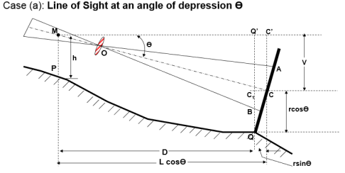
Fig-4 Line of sight at an angle of depression
In actual practice, observations may be made with either horizontal line of sight or with an inclined line of sight. In the latter case, the staff may be kept either vertically or normal to the line of sight. First, the distance-elevation formulae for the horizontal sights should be derived.
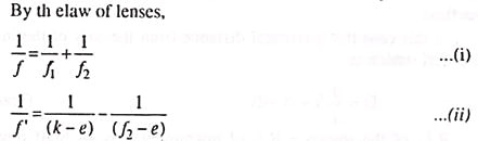
4.4 Anallatic Lens In External Focusing Telescope
An additional convex lens, called an analytic lens, is provided in an external focusing telescope between the eyepiece and object-glass at a fixed distance from the later, to eliminate the additive constant, (f+d), from the distance formula:

to simplify the calculation work. The analytic lens is seldom placed in internal focussing telescope since the value of the additive constant is only a few centimetres and can be neglected. The disadvantage of the analytics a lens is a reduction in the brilliancy of the image due to increasing observation of light.
The value of the additive constant, (δ+d) can be made equal to zero by bringing the apex (G) of geometric angle AGB (Fig. 10. 4) into exact coincidence with the centre on\f the instrument.
The theory of analytic lens is explained as follows:
|

Let, S = the staff intercept AB.
i = the length of the image of AB i.e. the actual stadia interval when the analytic lens is interposed.
i = the length ba of the image of AB when no analytic lens was provided.
O = the optical centre of the object-glass.
O = the optical centre of the analytic lens e = the distance between the optical centre of the object-glass and the analytic lens.
f = to cel length of object-glass.
f’ = focal length of the analytic lens.
F = Principle focus of the analytic lens.
G = the centre of the instrument.
d = the distance from the centre of the object-glass top the vertical axis of the instrument.
D – the distance from the vertical axis of the instrument to the staff.
f1and f2 = the conjugate focal length of the object-glass.
k = the distance from the optical centre of the object-glass to the actual image b a.
(k— e) and (f2 —e) = the conjugate focal length of the analytic lens.
The ray of light from A and B are refracted by the object-glass to meet at F. The analytic lens is so placed that F is its principal focus. Thus ray of light would become parallel to the axis of the telescope after passing through the analytic lens and give actual image b an of the staff intercept AB.
Refrence-2
The negative sign is used in (ii) since b ‘a’ and ba are on the same side of the analytic legs.
Refrence-3
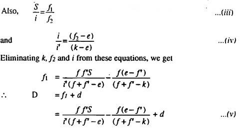
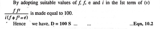
now the conditions that D should be proportional to S requires that the 2nd and 3rd terms in (v) are equal to zero so that
Refrence-4
In this condition, the apex G of the tacheometric angle AGB exactly coincides with the instruments
|

Refrence-5
In this condition, the apex G of the tacheometric angle AGB exactly coincides with the instruments
Refrence-6
Reduction of Readings:
In practice, horizontal and vertical distances are not calculated by the direct application of formulae, since it is much laborious.
But they are found by following means which are also based on these formulae:
(i) Taceometric tables.
(ii) Stadia diagrams.
(iii) Stadia slide rule.
The calculation work is also much reduced by the use of direct-reading tachometers.
(i) Tacheometric Tables:
There are various forms of geometric tables published by different authorities. The tacheometric tables which are in common use have been at end of the book as Appendix I. They provide horizontal and vertical distances for one metre of staff intercept when the multiplying constant of the instrument = 100 and the additive constant = 0.
The modern tachometer which is fitted with the analytic lens gives these values of the constants, the horizontal distance for 1m staff intercept;

and vertical distances for 1m staff intercept

The tables provided these values for different values of varying from 0° to 30°
For example, suppose, the vertical angle is 3° 20^ and the staff intercept is 1.70m. From the tables, it is seen that horizontal and vertical distance for 1-metre staff in percept i.e.

Thus for 1.70m staff intercept, the horizontal distance = 1.70 x 99 .67 – 169.439 m and the vertical distance = 1.70 x 5.80 = 9.86 m.
(ii) Stadia Diagrams:
The stadia diagrams show graphically the quantities

The diagram is available in different forms but surveyors often prepare these diagrams of their design. The use of stadia diagram is considered faster than the use of tables but can be used for ordinary distance.
iii) Stadia Slide Rule:
The horizontal and vertical distances are computed conveniently by stadia slide rule. Stadia slide rules are available in different patterns but one in common use is constructed like the ordinary slide rule, except that on slide rule are given values of cos2 and 1/2 sin 2, these qualities being plotted to a log scale. The stadia slide rule is equally suitable for field or office work.
Line of sight or line of collimation is the line passing threw intersection of horizontal and vertical crosshairs and the optical centre of objective glassy focusing the eyepiece for the distanced vision of crosshair. By focusing the objective to bring the image formed by the objective in the plane of crosshairs.
Focusing the Eyepiece
To focus the eyepiece, use the following procedure.
1. Keep a piece of white paper in front of the telescope or direct telescope towards a clear portion of the sky.
2. Looking through the telescope, adjust vision by rotating the eyepiece till the crosshairs come into sharp and clear view.
3. If the eyepiece has graduations, note the graduation at which you get a clear view of the crosshairs. This can help in later adjustment if required.
Levelling by Stadia:
Levelling by stadia tachometer is an indirect and rapid method of levelling. It is suitable where the country is rough and precision needed is not great. The transit should preferably be provided with a sensitive control level for vertical vernier so that error may be readily eliminated.
The method of running a line of levels by this method is as follows:
(i) Set up transit at a convenient point.
(ii) Take a backsight on the staff held at a B.M., first by observing stadia interval and then by measuring the vertical angle to some arbitrarily chosen mark on the staff.
(iii) Establish a change point in advance of transit, and take similar observations, the vertical angle is measured with horizontal cross-hair set on the same mark as before.
(iv) Move trait to a new point in advance of change point and repeat the process.
(v) Record stadia distance and vertical angles and also staff reading which is used as an index when vertical angles are measured.
STADIA REDUCTION FORMULAS.—
In stadia work we are concerned with finding two values as follows: (1) horizontal distance from the centre of the instrument to the stadia rod and (2) vertical distance, or elevation difference, between the centre of instrument and middle-hair reading on the rod. To obtain these values, you must use stadia reduction formulas.
Stadia Formula for Horizontal Sights.— For a horizontal sight, the distance that we need to determine the horizontal distance between the centre of the instrument and stadia rod. This distance is found by adding the stadia distance to instrument constant as follows:
Write ks for the stadia distance and (f + c) for instrument constant. Then the formula for computing horizontal distances when sights are horizontal becomes the following:
H=ks +(f+c)
Where:
h=horizontal distance from the centre of the instrument to a vertical stadia rod
k=stadia constant, usually 100
s=stadia interval
f + c =instrument constant (zero for internally focusing telescopes; approximately 1 foot for externally focusing telescopes)
f =focal lengths of the lens
c=distance from the centre of the instrument to the centre of the lens
The focusing eyepiece is the operation of bringing the crosshairs to focus. The focusing position varies with the eyesight of the observer. If the same observer taking the readings, this has to be done only once
The Tangential System of Tacheometry:
This method is used when the telescope is not fitted with a stadia diagram. In this method, the telescope is directed towards staff to which the horizontal and vertical distances are to be measured and two vertical angles to two vanes or targets on the staff at a known distance (S) apart are taken.
The horizontal and vertical distances are then calculated as follows:
Case 1:
When both the observed angles are angles of elevation:
|
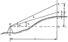
Fig-6 When both the observed angles are angles of elevation
In fig, let
O=The instruments station.
O’=The position of the instruments axis
P= The staff station.
∠AO’Q= θ1= vertical angle to the upper vane.
∠BO’Q= θ2 =” “ “ lower
AB=S=the staff intercept.
BQ=V= the horizontal distance from the inst, axis to the lower vane.
O’Q=D= the horizontal distance from the inst. station O to the staff station P
PB= h= the height of the lower vane above the foot of the staff.
Refrence-7
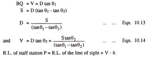
Case II:
When both the observed angles are angles of depression: (Fig. 10.11).
|
Refrence-8
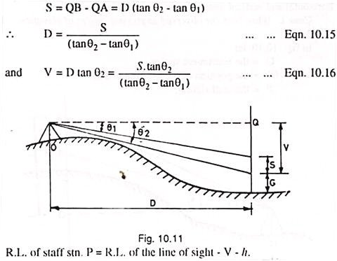
Case III.
When one of the observed angles is the angle of elevation and the other an angle of depression:
|
Refrence-9
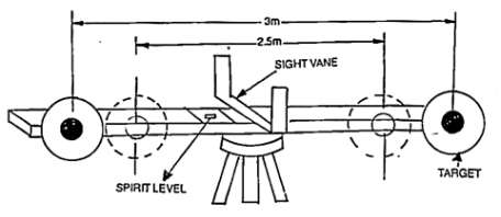
A subtense bar (fig. is a horizontal staff with targets fixed at a known distance apart. It is about 4m long having a small spirit level and a quick levelling head.
A sight rule, provided at its centre, can be placed along the line of sight by viewing the telescope of the theodolite thought the vanes. The bar is mounted on a tripod and is placed at right angles to the line of sight for making observations. After levelling and aligning, it is clamped using a clamp screw.
The targets, made of discs of about 20 cm diameter are painted red on one side, and white on the other. The centres of body sides of the targets are painted black in 7.5 cm diameter. The targets are placed at a distance of 2.5 m and 3 m. When targets are placed 2.5 m apart, the white faces are to face instrument and when they are placed 3m apart, the red faces face instrument.
|
The horizontal and vertical angles are measured with a transit theodolite. For measuring vertical angles method will be similar to the movable hair method of stadia tachometer and distances are similarly deduced. For measuring horizontal angles, subtended at the instrument station by two targets, the method of repetition is used, the horizontal distance.
D between the instrument station and the subtense bar station is found as follows:
Let O= the position of the instrument for measuring the horizontal angle 0 by the horizontal circle of the theodolite.
AB= horizontal base of a length S.
|
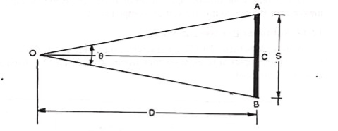
Fig-8 D between the instrument station and the subtense bar station
|

Refrence-10
subtense bar was used to allow the quick measurement of distances, by measuring the angle that the subtense bar subtended at the theodolite observing it.
It is the type of graduated arc attached to the vertical circle of an alidade or transit to make the computing elevation difference for inclined stadia sights simply.
The arc, designed by W. M. Beaman of the U. S. Geological Survey, is that each division on the arc is equal to 100 (1/2 sin 2A),
where A = vertical angle.
the index is set exactly on graduation and difference in height along an inclined line of sight is obtained by multiplying the stadia intercept by the number of Beaman arc divisions
|
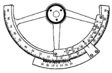
the index is set exactly on graduation and the difference in elevation along an inclined line of sight is obtained by multiplying the stadia intercept by the number of Beaman arc divisions.
Reference:
1 Madhu, N, Sathikumar, R and Satheesh Gobi, Advanced Surveying: Total Station, GIS and Remote Sensing, Pearson India, 2006.
2 Manoj, K. Arora and Badjatia, Geomatics Engineering, Nem Chand & Bros, 2011
3 Bhavikatti, S.S., Surveying and Levelling, Vol. I and II, I.K. International, 2010
4 Chandra, A.M., Higher Surveying, Third Edition, New Age International (P) Limited, 2002.
5 Anji Reddy, M., Remote sensing and Geographical information system, B.S.


