When two straight lines intersect at some angle then a curve is provided in between them which meets the straight line tangentially.
Necessity (Curves are provided for the following reasons)
- Curves are needed on highways Railways and Canal for bringing about a gradual change of direction of motion
- to bring about gradual changes in direction of motion
- to connect important places
- to avoid obstructions
- to bring about gradual changes in grade and for good visibility
- to balance earthquake in acceleration cutting
- minimising construction cost
|
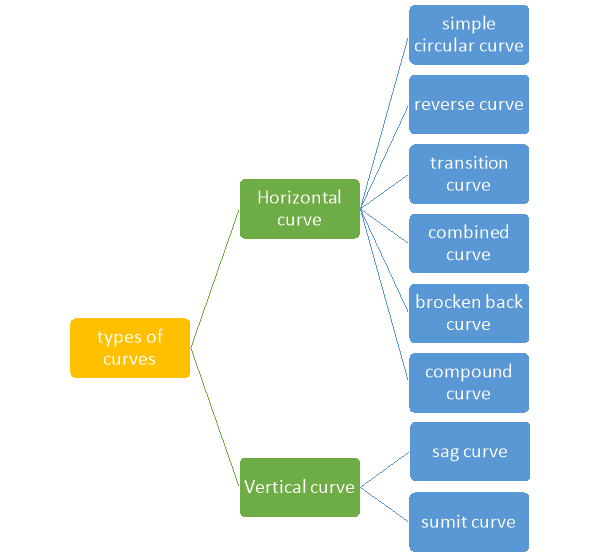
Table 1 types of curves
The curve is in fact Arc with some definite radius and centre that is they are a part of the circle. it is due to the curves only that the change in direction is made possible a very smooth task
|
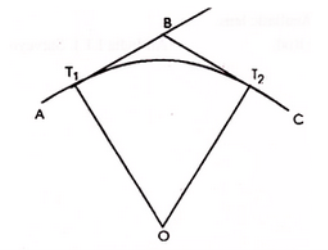
Fig-1 simple curves
- the simple curve consists of a single arc of a circle connecting two straights.
- It consists radius of the same magnitude throughout.
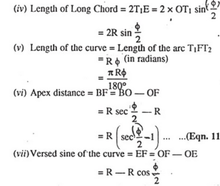
- T1 D T2 is the simple curve with T1O as its radius
|
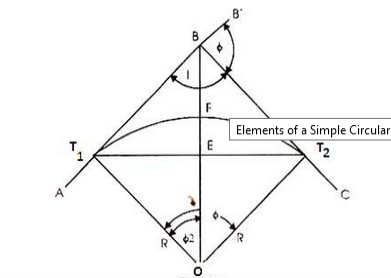
Fig-2 element of simple curves
|
|
A simple curve consists of a single arc of a circle connecting two straights. In simple closed curves the shapes are closed by line-segments or by a curved line. Triangle, quadrilateral, circle, etc., are examples of closed curves.
A curve may be designated either by the
- radius or
- angle (in degrees) subtended at the centre by a chord of 30 metres (100 ft.) length.
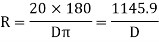
The relation between degree and radius of the curve.
Arc definition / Chord Definition:-
Arc definition of degree of the curve: According to this, degree of curve in the central angle subtended by an arc of the length of 20m or 30 m.
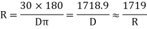
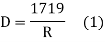
If R = radius of curve
D = degree of curve as per arc definition for 30m arc length.
D° = 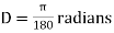
Q (radians) = 
For 20 mm length
|


Method of setting out curve
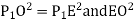
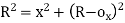
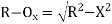
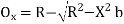
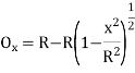
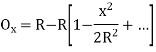
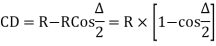
- The linear method offset from long chord
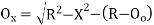
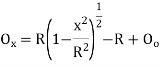
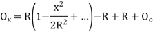
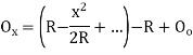
Where 
 offset at some point P at distance x from midpoint D.
(ii) Perpendicular offset from tangent
|
Fig-3 linear method offset from long chord

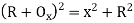
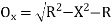
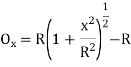
(iii) Radial offset from tangent:
|
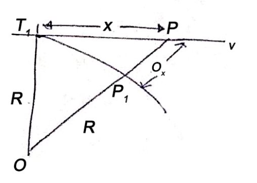
Fig-4 Radial offset from tangent:

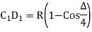
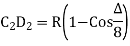
(iv) Successive Bisection of Arc or chord
|
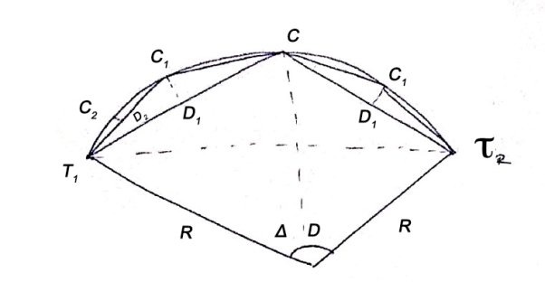
Fig-5 Successive Bisection of Arc or chord
(v) By offset from chord produced
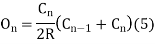
 last sub chord
b) Angular method
i) Rankine's method of the deflection angle
- It is generally used for setting out a circular curve of long length and large radius.
- It gives good result except then chords are long as compared to a radius, so that variation between the length of an Arc and its cord becomes considerable.
- It is used in highway and Railway
 = Tangential angle
C = chord length
(ii) Tacheometric method
-It is similar to Rankine’s method of deflection angle.
- The theodolite at may be used as Tacheometric and Tacheometric observation are made.
- Less accurate as compared to Rankins.
- Chaining is completely dispersed in this method.
(For Incline and line of sight)
(For the horizontal line of sight)
- Two theodolite method
- Convenient than any of our method when the ground is undulating rough and not suitable for Linear measurements.
- Two theodolites are used and linear measurement is eliminated.
- Hence, the most accurate method.
- It is based on the principle that the angle between the tangent and chord is equal to the angle subtended by a chord in the opposite segment.
- Time-consuming method
- Most accurate method
- Highly expensive.
To establish the first curve station, first set the horizontal circle reading of the instrument to zero and sight along the back tangent.
In this method, curves are staked out by use of deflection angles turned at the point of curvature from tangent to points along the curve. The curve is set out by driving pegs at a regular interval equal to the length of a normal chord. Usually, sub-chords are provided at the beginning and end of the curve to adjust the actual length of the curve. The method is based on assumption that there is no difference between the length of the arcs and their corresponding chords of normal length or less. The underlying principle of this method is that deflection angle to any point on the circular curve is measured by one-half the angle subtended at the centre of the circle by the arc from the P.C. to that point. [Rule 1 under "Fundamentals of the geometry of the Circular Curve" stated in lesson 37].
Let pts a,b,c,d,e are to be identified in the field to lay out a curve between T1 and T2 to change direction from the straight alignment AV to VB
.
|
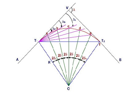
Fig-6 Rankine’s deflection angle method
To decide about points, chords ab, bc, cd, de are being considered having the nominal length of 30m. To adjust the actual length of curve two sub-chords have been provided one at the beginning, T1 a and other, eT2 at end of the curve. The number of deflection angles that are to be set from the tangent line at the P.C. is computed before setting out the points. The steps for computations are as follows:
|
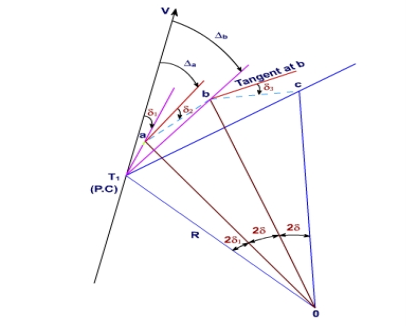
, Fig-7 Rankine’s deflection angle system
let the tangential angles for points a, b, c,… be d1, d,…, d, dn and their deflection angles (from the tangent at P.C.) be Da, Db, ….., Dn.
Arc T1 a = R x 2d1 radians
Assuming the length of the arc is same as that of its chord if C1 is the length of the first chord i.e., chord T1 a, then

(Note: the units of measurement of chord and that of the radius of the curve should be same).
Similarly, tangential angles for chords of nominal length, say C,

And for the last chord of length, say Cn

The deflection angles for the different points a, b, c, etc. can be obtained from tangential angles. For the first point a, deflection angle Da is equal to the tangential angle of the chord to this point i.e., d1. Thus,
Da =d1.
The deflection angle to next point i.e., b is Db for which the chord length is T1 b. Thus, the deflection angle

Reference -6
Thus, the deflection angle for any point on the curve is deflection angle up to the previous point plus tangential angle at the previous point.
Rankine's method is a technique for laying out circular curves by a combination of chaining and angles at circumference
CURVE SETTING (Compound and Reverse curves)
The compound curve is a combination of curves of two or more radii.
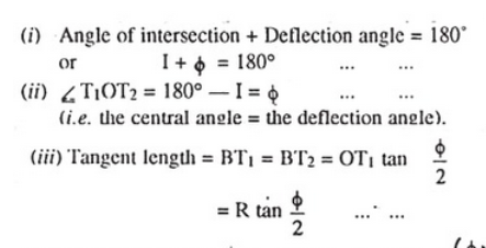
Elements
The compound curve has seven elements
- Radius R1,
- Radius R2,
- deflection angle φ,
- the deflection angle of the first arc φ1,
- the deflection angle of the second arc φ2,
- tangent length LT1 and LT2.
Elements of Compound Curves
∆ = ∆ 1 + ∆ 2
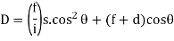
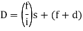
IT1 = T1M + MI = R1 tan ∆ 1 /2 + MN sin ∆ 2 /sin ∆ IT2 = T2N + NI = R2 tan ∆ 2 /2 + MN sin ∆ 1 /sin ∆ 2
|
Design of compound curves
Compound Curve between Successive PIs
The calculations and procedure for laying out a compound curve between successive PIs are outlined in the following steps. This procedure is illustrated in figure 11a.
|
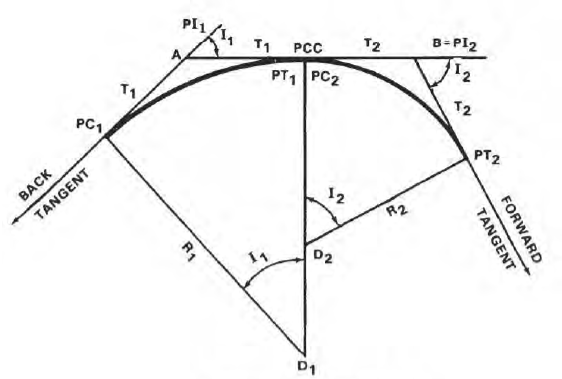
Fig-9 Design of compound curves
FIGURE Between Successive PIs – Compound curves
- Find out the PI of the first curve at point A from field data or last computations.
- make I1, I2, and distance AB from the field data.
- Find the value of D1, the D for the first curve.
- Compute R1, the radius of the first curve
- find T1, the tangent of the first curve.
- T1 = R1(Tan ½ I)
- find T2, the tangent of the 2ndcurve.
- T2 = AB – T1
- findR2, the radius of the 2nd curve.
- R2 = T2 / Tan ½ I
- findD2 for the second curve...
- Compare D1 and D2. They should not differ by more than 3 degrees, if not then check again
- If the two Ds are fine, then compute the remaining data and deflection angles for the first curve.
- Compute the PI of the second curve. Since the PCC is at the same station as the PT of the first curve, then PI2 = PT1 + T2.
- Compute the remaining data and deflection angles for the second curve, and lay in the curves.
Compound Curve between Successive Tangents. Place the instrument at the PI and sight
along the back tangent.
- Layout a distance AC from the PI along the back tangent, and set PI1.
- See the back tangent from PI2 a distance T1, and set PC1.
- Sight along the forward tangent with the instrument still at the PI.
- Layout a distance BC from the PI along the forward tangent, and set PI2.
- see along the forward tangent from PI a distance T2, and set PT2.
- Check the location of PI1 and PI2 by either measuring the distance between the two PIs and comparing the measured distance to the computed length of line AB, or by placing the instrument at PI1, sighting the PI, and laying off I1. The resulting line-of-sight should meet PI2.
Design procedure of compound curves
Step 1: Locate tangent point T, by measuring back the total tangent length (Tt) along the back tangent, from the point of intersection V.
Likewise, locate the tangent point T' by measuring along forward tangent the distance Tt from V.
Setting out of transition curve :
Step 2: Set a theodolite over the point T. Set vernier A to zero, and clamp the upper plate.
Step 3: Direct the line of sight of theodolite to intersection point V, and clamp lower plate.
Step 4: Release upper plate. Set the vernier A to first deflection angle (a1).
The line of sight now points towards the first peg on the transition curve.
Step 5: With the zero of the tape pinned at T and an arrow kept at mark corresponding to the first length of the chord, the assistant will swing the tape till the arrow is bisected by a line of sight.
Fix the first peg at arrow point.
Step 6: Set the vernier A on the second deflection angle (a2) to the direct line of sight to the second peg.
Step 7: With zero of the tape pinned at T, and keeping an arrow at mark corresponding to the total length of the first and second chords, the assistant will swing an arc till the arrow is bisected by the line of sight.
Fix the second peg at arrow point. It should be remembered that the distance is measured from the point T and not from the preceding point.
Step 8: Repeat steps (6) and (7) till the last point C on the transition curve is reached.
Setting out of the circular curve :
Step 9: For setting out circular curve CC', shift the theodolite to junction point C.
Orient theodolite concerning the common tangent CC1 by directing the line of sight towards CT with vernier. A set at a reading equal to , and swinging the telescope clockwise in azimuth by fs(Figure 39.4).
Now the line of sight is directed along the common tangent CC1 and the vernier reads zero.
Step 10: Plunge telescope. The line of sight is now directed along the tangent C1C produced.
deflection angles D1, D2, etc. have been calculated concerning the tangent C1C produced at C (Figure 38.2).
The line of sight is now correctly oriented, and reading of the vernier A is zero.
Step 11: Set the vernier A to first deflection angle D1, and locate the first peg on the circular curve at a distance of c' from C, where c' is the length of the first sub-chord.
Step 12: Likewise, locate the second peg on the circular curve at the distance c equal to the normal chord from the first peg with the deflection angle D2 at C.
Step 13: Continue the above process till junction point C' is reached.
Step 14: Set out the transition curve TC' from T' using the same procedure as that for transition curve TC.
Since their tangent lengths vary, compound curves fit the topography much better than simple curves. These curves easily adapt to mountainous terrain or areas cut by large, winding rivers. However, since compound curves are more hazardous than simple curves, they should never be used where a simple curve will do.
Setting out of compound curves
Setting a compound curve
- Calculate all elements ∆1, ∆2, ∆, R1, R2, IT2 and IT1.
- Locate PI (I), PC (T1) and PT (T2)
- Calculate chainage of T1 (chainage of I – tangent length IT1)
- Calculate chainage of the point of compound curvature D.
- Chainage of D = Chainage of T1 + length of arc T1D = chainage of T1 + ΠR1 ∆1 / 180o
- Calculate chainage of T2 = chainage of D + ΠR2 ∆2 / 180o
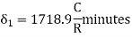
- Calculate the deflection angles for both the arcs from their tangents, e.g. ∆1 = δ1 = 1719 C1 / R, where C1 is the chord length and R is the radius
These curves are used in direction change for the roadways and it includes the interchange ramps. It is used to provide the layout of canal alignment.
Reverse curve between two parallel straights (Equal radius and unequal radius).
Reverse curve:-
When to normal circular curves of different or equal radii, have opposite in direction of curvature join together, the formed or resultant curve is known as a reverse curve.
Uses:-
- When the angle between the two straight lines is very small.
- When two straight lines are parallel to each other.
The element of a reverse curve
|
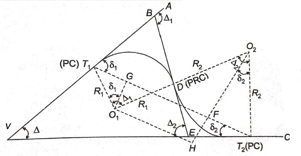
Fig-10 Element of reverse curve
- VA and uc include deviation angle of - - - - Join |


In ∆BVE,


In 

From (1) and (2)

In, 
In,
|


Also,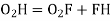
From (3) and (4)
|


Element of Reverse Curve / Reverse Curve Between two parallel straight
In ∆BVE
∆1 = ∆ + ∆2
∆ = ∆1 - ∆2
In ∆ T1VT2
S1 = ∆ + S2
∆ = S1 – S2
∆1 - ∆2 = S1 – S2
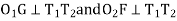
O1G ∥ O2P
∆1 – S1 = ∆2 – S2
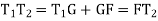
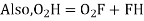
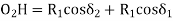
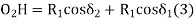
∆1 - ∆2 = S1 – S2 In ∆T1GO1 T1G = R1 sin δ1 , O1G = R1 cos δ1 In ∆T2FO2 T2F = R2 sin δ2 , O2F = R2 cos δ2 GF = O1H = (R1 + R2) sin (∆2 – δ2) T1T2 = T1G + GF + FT2 = R1 sin δ1 + (R1+ R2) sin (∆2 – δ2) + R2 sin δ2 O2H = O2F + FH = O2F + FH = O2F + O1G |
= R2 cos δ1 + R1 cos δ1 ...............................(1)
In ∆ O1O2 H
O2H = (R1+ R2) cos (∆2 – δ2) ................................(2)
From (1) and (2)
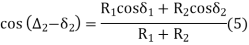
R2 cos δ2 + R1 cos δ1 = (R1 + R2) cos ( ∆2 – δ2)
cos ( ∆2 – δ2) = R2 cos δ2 + R1 cos δ1/ (R1 + R2) |
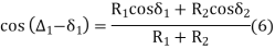
similarly
cos ( ∆1 – δ1) = R1 cos δ1 + R1 cos δ2/ (R1 + R2) |
The reverse curve is useful when laying out of pipeline, flumes, and levees. the surveyor may also use them on low-speed roads and railroad
Reference:
1 Madhu, N, Sathikumar, R and Satheesh Gobi, Advanced Surveying: Total Station, GIS and Remote Sensing, Pearson India, 2006.
2 Manoj, K. Arora and Badjatia, Geomatics Engineering, Nem Chand & Bros, 2011
3 Bhavikatti, S.S., Surveying and Levelling, Vol. I and II, I.K. International, 2010
4 Chandra, A.M., Higher Surveying, Third Edition, New Age International (P) Limited, 2002.
5 Anji Reddy, M., Remote sensing and Geographical information system, B.S.


