UNIT - 7
CURVE SETTING (Transition and Vertical curves)
- It is a curve introduced between a simple circular curve industry tour between two simple circular curves.
- Also known as easement curve.
- Its videos, gradually changing from a finite to infinite value or vice versa.
- It is generally used in highway and Railway.
To minimize the effects of centrifugal force, the speed of the vehicle should be gradually reduced or a path should be negotiated with the gradual change of trajectory so that the radius of curvature is gradually reduced from infinity to R or to get the combined effect of both.
The element of the Transition curve
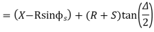
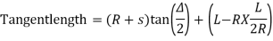
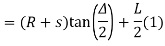
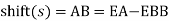
(a)Total Tangent Length
|
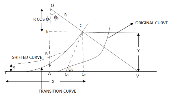
Fig-1 Tangent length
Tangent length
|

(b) Length of the long chord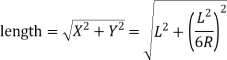
(c) Total length of the curve
|
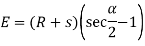
(d) Apex distance E


Key takeaway
Transition curves are curves in which the radius changes from infinity to a particular value. The effect of this is to gradually increase the radial force P from zero to its highest value and thereby reduce its effect.
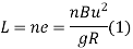
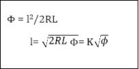
Length of transition curve:-
Method of arbitrary gradient:-e = total super elevation provided at the junction of transition curve with the circular curve
L = ne
Where the rate of superelevation is ∆ in n

(b) Method of Time rate:-
the time rate of superelevation


Method of the rate of change of radial acceleration
Rate of change of radial acceleration
t is the time attained by radial acceleration (a)
a = 


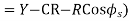
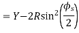
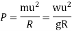
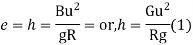
Superelevation or Cant:
It is defined as the raising of the outer end of a road or outer rail over the inner one.
h = super elevation = e
w = weight of the vehicle
P = centrifugal force
g = acceleration due to gravity
R = radius of the curve
G = gauge distance between rails
u = speed of the vehicle
B = width of pavement
= Angle of superelevation
h = super elevation = e
w = weight of vehicle
P = centrifugal force
g = acceleration due to gravity
R = radius of curve
G = gauge distance between rails
u = speed of vehicle
B = width of pavement
= Angle of super elevation


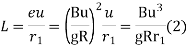
 Centrifugal ratio
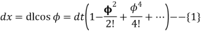
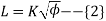
Let there is point distance 𝛿l from B. Thus the coordinates of P are (x+ 𝛿x) and (y+ 𝛿y). The Tangent Pρ1 at P makes an angle of
(ϕ + 𝛿ϕ)with the initial tangent TD.
|

|
Differentiating above equation
dl=K/ ×dΦ----{3}
Putting in equation 1-
dx = K/ ×( ) dΦ
∝x = k/2 ( ϕ-1/2 – ϕ3/2/2b + ϕ7/2/4b - ......)
Integrating, we get x = k/2 (2 ϕ1/2 – ϕ5/2/5 + ϕ7/2/108 - ......) x= k ( 1 – 1/10 ϕ2 + ϕ4/ 216 - ......) l = k x = l ( 1 – 1/10 ϕ2 + ϕ4/ 216 - ......) (l = k ) x= l (1 – l4/10k4 + l8/216k - ....) k = (also) x = l( 1 – l4/ 40 R2L2 + – l8/ 3456 R2L8 - ...) |
similarly expression for y can be obtained as follows:-
δy/δl = sin ϕ dy = dl sin ϕ = dl ( ϕ – ϕ3/3! + ϕ5/5! - ...) dl = k/ 2 dϕ dy = dl sin ϕ = dl ( ϕ – ϕ3/3! + ϕ5/5! - ...) dy = k/2 (ϕ1/2 - ϕ5/2/3! + ϕ3/2/5! - ...) dϕ |
Integrating, we get
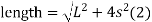
y = k (ϕ3/2/3 – ϕ7/2 /42 + ϕ11/2 /1320 - ......) dϕ l = k y = l3/3k2 ( 1 – l4/14 k4 + l8/ 440 k8 - ...) dϕ y = l3/6RL ( 1 – l4/56 R4 L4+ l8/ 7040 R4L4 - ...) dϕ
The cubic spiral
y = l3/6RL ( 1 – l4/56 R4 L4+ l8/ 7040 R4L4) |
Neglecting all terms
Beyond the first term
y = l3/6RL
if x = l
y = x3/6RL
if the equation is cubic parabola then sin ϕ≈ϕ
cos ϕ≈ 1
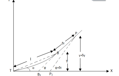
Setting out of Cubic Parabola
|
Fig-3 Setting out of Cubic Parabola
x = TM1 = distance of any point in an curve measured along tangent TB y = M1M = perpendicular offset to point M X = TE1 = distance of junction point E of transition curve Y = E1E = perpendicular offset to junction point E L = length of transition curve Φ = LMM2B = angle between AB & tangent to transition curve Φ1 = LEE2B = angle between TB & tangent E R = radius of curve ∝ = deflection angle to any point M ∝1 = deflection angle to junction E x = l y = l3/ERL = x3 / ERL .................................(1) ∝ = l2/ERL radian = 1800l2/πRL min |
∝ = 573 l3/RL min
..................................(2)
l= L also ∝n = 573 L/R min
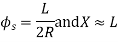
Φ1 = L/2R radians = 3 × 573 L/R min
.................................(3)
If R = 1719/D thin
∝ = Dl2/3L min
...................................(4)
&∝n = DL/3 min
Φ1 = DL min = θL/60 degree x = l ( 1 – Φ2/10) = l (1 – l4/40R2L2) ...................................(5) y = l3/6RL ( 1 – Φ2/14) = l3/6RL ( 1 – l4/ 14 (2RL)2) .............(6) X = L ( 1 - Φ12/10) = L ( 1 – L2/40 R2) = L ( 1 – 33/ 5R) ..........(7) Y = L2/ 6R ( 1 – L2/ 56 R2) |
Setting out of Bernoulli‟s Lemniscate
|
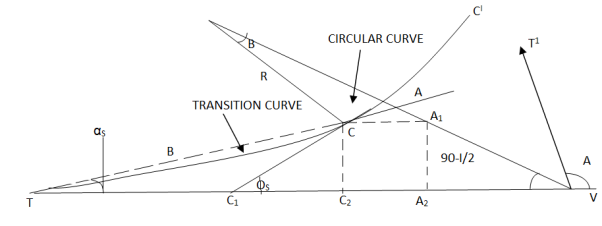
Fig-5 Setting out of Bernoulli‟s Lemniscate
∝s = Polar deflection angle
OU bisect the ∆TUT’ at vertex V Hence
TU & T’V are tangent of curve
Make CA1 parallel to tangent TV intersecting OU at A1
Draw CC2& A1A2 normal tangent TV
Φs = Total deflection angle at junction C
∠CTV = ∝s
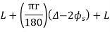
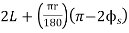
∠CC1V= Φs TV = TC2 + C2A2 + A2V (tangent length = TV) Length of chord, TC = B = ∝s = Φ/3 TC2 = B cos ∝s ∠TUo = (180° - ∆)/2 = 90° - ∆/2 In ∆AC1V1, ext ∠OAC = ∠AGV + ∠GVA = Φs + (90° - ∆/2) ∠AOC = 90° - ∠AOC = 90° - [Φs + (90° - ∆/2)] β = ∆/2 - Φs From ∆OCA1⇒ C0/CA1 = sin (90° - ∆/2)/sin (∆/2 - Φs) CA1 = R sin (A/2- Φs)/cos (∆/2) = R sec (∆/2) [ sin (∆/2) cos Φs - cos (∆/2) sin Φs] CA1 = C2A2 = R [ tan (∆/2) cos Φs – sin Φs] A2 V = A1A2 Cot (90° - ∆/2) = CC2 Cot (90° - ∆/2) = B sin ∝s tan (∆/2) Adding all equation TU = TC2 + C2A2 + A2V TU = B cos ∝s + R [ tan (∆/2) cos Φs – sin Φs ] + B sin ∝s tan ∝s |
The minimum rate of change of curvature is required for both heavy and light vehicles on the highway, and this necessitates the use of Lemniscate curves are used in highways
These are curves in a vertical plane, used to join two intersecting grade lines.
A vertical summit curve is provided when a rising grade join a failing grade and a vertical curve is provided when a falling grade joins a rising grade.
|
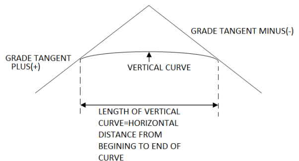
Fig-6 vertical curves
|
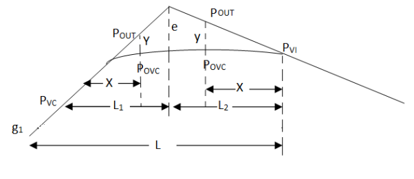
Fig-7 vertical curves Distribution
PVC – point of vertical curvature place where the curve begins
PVT – point of vertical tangency, where curve end.
PVI – point of vertical intersection, where grade tangents intersect.
POVC - a point on vertical curve applies to any point on the parabola
POVT - a point on a vertical tangent, applies to any point on other tangents
are grade tangent at PVC and PVT respectively.
Length of vertical curve
L = algebraic difference of two grades/ rate of change of grade

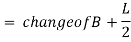
Change of end of the curve
PVT = change of intersection point + half the length
Types of vertical curves
Upgrade followed by a downgrade
|
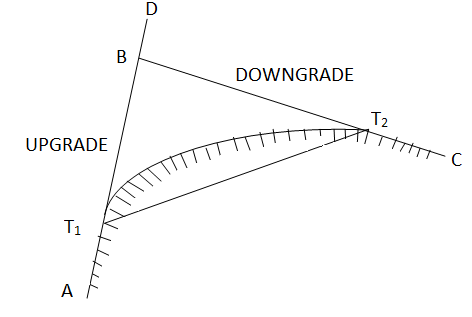
Fig-8 Upgrade followed by a downgrade
2.Upgrade followed by another upgrade
|
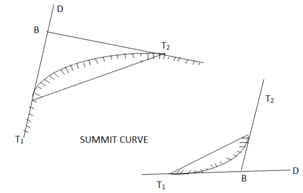
Fig-9 Upgrade followed by another upgrade
A downgrade followed by an upgrade
|
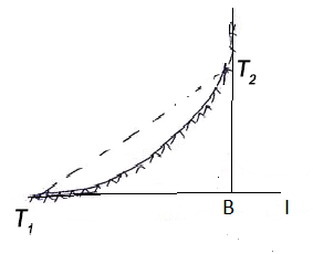
Fig-10 A downgrade followed by an upgrade
A downgrade followed by another downgrade
Vertical curves are used in highway and street vertical alignment to provide a gradual change between two adjacent grade lines.
Reference Books:
1 Madhu, N, Sathikumar, R and Satheesh Gobi, Advanced Surveying: Total Station, GIS and Remote Sensing, Pearson India, 2006.
2 Manoj, K. Arora and Badjatia, Geomatics Engineering, Nem Chand & Bros, 2011
3 Bhavikatti, S.S., Surveying and Levelling, Vol. I and II, I.K. International, 2010
4 Chandra, A.M., Higher Surveying, Third Edition, New Age International (P) Limited, 2002.
5 Anji Reddy, M., Remote sensing and Geographical information system, B.S.


