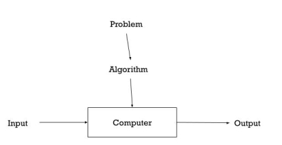
Basically, algorithms are the finite steps to solve problems in computers.
It can be the set of instructions that performs a certain task.
The collection of unambiguous instructions occurring in some specific sequence and such a procedure should produce output for a given set of input in a finite amount of time is known as Algorithm.
In addition, all algorithms must satisfy the following criteria:
● input: can be zero or more input
● output: must produce output
● finiteness: must have ending
● definiteness: unambiguous and clear
● effectiveness: should not be complex
|
Fig 1: about algorithm
A finite set of steps, each of which may require one or more operations, is composed of an algorithm. The probability of these operations being performed by a machine demands that certain restrictions be imposed on the type of operations that an algorithm might include. The fourth criterion we assume in this book for algorithms is that after a finite number of operations, they terminate.
Criterion 5 demands that each process be efficient; each step must be such that a person using pencil and paper can do it in a finite amount of time, at least in theory. An example of successful operation is the output of arithmetic on integers, but arithmetic with real numbers is not, since certain values can only be represented by infinitely long decimal expansion. The efficacy property will be violet when adding two such numbers.
● Computational procedures are often called algorithms that are definite and efficient.
● The same algorithm can be interpreted in many ways by the same algorithm.
● Many algorithms to answer the same problem
● Various different speed definitions
Euclid’s algorithm -gcd (m, n) =gcd (n,m mod n) Until m mod n =0, since gcd(m,0) =m
|
Euclid’s algorithm
Step1: Assign the value of min (m, n) to t Step 2: Divide m by 5t. if remainder is 0, go to step3 else goto step4 Step 3: Divide n by t. if the remainder is 0, return the value of t as the answer and stop, otherwise proceed to step4 Step4: Decrease the value of t by 1. go to step 2 |
Key takeaways
- Basically, algorithms are the finite steps to solve problems in computers.
- It can be the set of instructions that performs a certain task.
- A procedure should produce output for a given set of input in a finite amount of time is known as Algorithm.
Following are the conditions where we can analyse the algorithm:
● Time efficiency: - indicates how fast algorithm is running
● Space efficiency: - how much extra memory the algorithm needs to complete its execution
● Simplicity: - generating sequences of instruction which are easy to understand.
● Generality: - It fixes the range of inputs it can accept. The generality of problems which algorithms can solve.
It is a formal way to speak about functions and classify them.
It is used to specify the running time and space complexity of an algorithm and to frame the run time performance in mathematical computation.
It refers to boundation or framing into the mathematical terms.
As the algorithm has three cases according to time taken by program to perform a certain task.
- Worst case: Performance (number of times performed by the specific operation) for Input of the worst-case size n. I.e.-I.e. Of all possible inputs of size n, the algorithm runs the longest.
- Best case: Performance (number of times performed by the specific operation) for the Input best case size n. I.e.-I.e. Among all possible inputs of size n, the algorithm runs the fastest.
- Average case: Average time taken (number of times it would take for the basic operation Executed) to address all possible instances of the input (random).
Following are the asymptotic notations which are used to calculate the running time complexity of algorithm:
- Big Oh (O) notation
- Big Omega (ῼ) notation
- Theta (Ꙫ) notation
Big Oh (O) Notation:
● It is the formal way to express the time complexity.
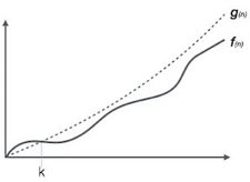
● It is used to define the upper bound of an algorithm’s running time.
● It shows the worst-case time complexity or largest amount of time taken by the algorithm to perform a certain task.
|
Fig 2: Big Oh notation
Here, f (n) <= g (n) …………….(eq1) where n>= k, C>0 and k>=1 if any algorithm satisfies the eq1 condition then it becomes f (n)= O (g (n)) |
Big Omega (ῼ) Notation
● It is the formal way to express the time complexity.
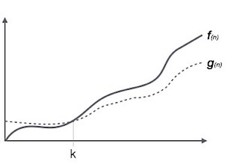
● It is used to define the lower bound of an algorithm’s running time.
● It shows the best-case time complexity or best of time taken by the algorithm to perform a certain task.
|
Fig 3: Big omega notation
Here, f (n) >= g (n) where n>=k and c>0, k>=1 if any algorithm satisfies the eq1 condition then it becomes f (n)= ῼ (g (n)) |
Theta (Θ) Notation
● It is the formal way to express the time complexity.
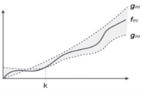
● It is used to define the lower as well as upper bound of an algorithm’s running time.
● It shows the average case time complexity or average of time taken by the algorithm to perform a certain task.
|
Fig 4: Theta notation
Let C1 g(n) be upper bound and C2 g(n) be lower bound.
C1 g(n)<= f (n)<=C2 g(n)
Where C1, C2>0 and n>=k
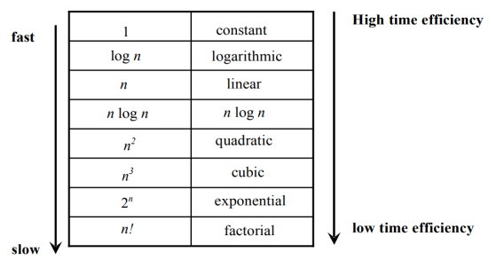
Basic Efficiency classes
The time efficiencies of a large number of algorithms fall into only a few classes
|
Key takeaways
- Big Oh is used to define the upper bound of an algorithm’s running time.
- Big Omega is used to define the lower bound of an algorithm’s running time.
- Theta is used to define the lower as well as upper bound of an algorithm’s running time.
Mathematical analysis (Time efficiency) of Non recursive algorithm.
General plan for analyzing efficiency of non-recursive algorithms:
- Decide on parameter n indicating input size
- Identify algorithm ‘s basic operation
- Check whether the number of times the basic operation is executed depends only on the input size n. If it also depends on the type of input, investigate worst, average, and best-case efficiency separately.
- Set up summation for C(n) reflecting the number of times the algorithm ‘s basic operation is executed.
- Simplify summation using standard formulas.
Example 1:
Finding the largest element in a given array ALGORITHM MaxElement(A[0..n-1]) //Determines the value of largest element in a given array //Input: An array A[0..n-1] of real numbers //Output: The value of the largest element in A currentMax ← A[0] for i ← 1 to n - 1 do if A[i] > currentMax currentMax ← A[i] return currentMax |
Analysis:
- Input size: number of elements = n (size of the array)
- Basic operation:
● Comparison
● Assignment
3. No best, worst, average cases.
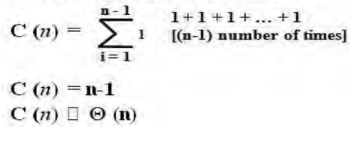
4. Let C (n) denotes number of comparisons: Algorithm makes one comparison on each execution of the loop, which is repeated for each value of the loop ‘s variable I within the bound between 1 and n – 1.
|
5. Simplify summation using standard formula
|
Example 2: Element uniqueness problem
Algorithm UniqueElements (A[0..n-1]) //Checks if all elements are distinct in a given array //Input: An array A[0..n-1] //Output: If all the elements in A are distinct and false otherwise, returns true for i 0 to n - 2 do for j i + 1 to n – 1 do if A[i] = = A[j] return false return true |
Analysis
- Input size: number of elements = n (size of the array)
- Basic operation: Comparison
- Best, worst, average cases EXISTS.
An array giving the largest comparisons is the worst case input.
● Array without identical elements
● The only pair of equivalent elements is the series of the last two elements.
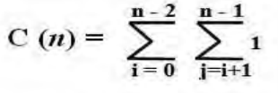
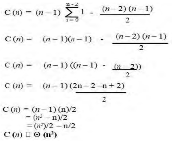
4. In the worst case, let C(n) denote the number of comparisons: for each repetition of the innermost loop, the algorithm makes one comparison, i.e., for each value of the loop variable j between its limits I + 1 and n-1; and this is repeated for each value of the outer loop, i.e. for each value of the loop variable I between its limits 0 and n-2.
|
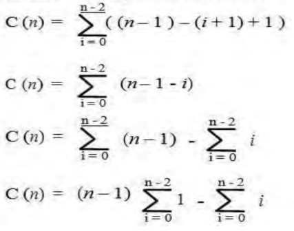
5. Simplify summation
|
|
Mathematical analysis (time efficiency) of recursive algorithm
General plan for analysing efficiency of recursive algorithms:
- Decide on the n parameter that indicates the input size.
- Identify the basic operation of an algorithm.
- Check that the number of times the basic operation is performed depends only on the size of the input n. If it also relies on the type of input, separately investigate worst, average, and best-case performance.
- Set up a recurrence relationship for the number of times the basic operation of the algorithm is executed, with a suitable initial condition.
- Solve the repetition.
Example 1: Factorial function
//Computes n! recursively //Input: A nonnegative integer n //Output: The value of n! if n = = 0 return 1 else return Factorial (n – 1) * n Analysis 1. Input size: given number = n 2. Basic operation: multiplication 3. NO best, worst, average cases. 4. Let M (n) is number of multiplications. M (n) = M (n – 1) + 1 for n > 0 M (0) = 0 initial condition Where, M (n – 1) : to compute Factorial (n – 1) 1 :to multiply Factorial (n – 1) by n 5. Resolve the recurrence: Resolving using "Method of backward substitution": M (n) = M (n – 1) + 1 = [ M (n – 2) + 1 ] + 1 = M (n – 2) + 2 = [ M (n – 3) + 1 ] + 3 = M (n – 3) + 3 … In the ith recursion, we have = M (n – i ) + i When i = n, we have = M (n – n ) + n = M (0 ) + n Since M (0) = 0 = n M (n) = Θ (n) Example 2: In the binary representation of a positive, find the number of binary digits Decimal Integer Integers ALGORITHM BinRec (n) //Input: A positive decimal integer n //Output: In n”s binary representation, the number of binary digits if n = = 1 return 1 else return BinRec (└ n/2 ┘) + 1 Analysis
A (n) = A (└ n/2 ┘) + 1 for n > 1 A (1) = 0 initial condition Where: A (└ n/2 ┘) : to compute BinRec (└ n/2 ┘) 1: to increase the returned value by 1 5. Solve the recurrence: A (n) = A (└ n/2 ┘) + 1 for n > 1 Assume n = 2k (smoothness rule) A (2k ) = A (2k-1) + 1 for k > 0; A (20) = 0 Solving using "Method of backward substitution": A (2k ) = A (2k-1) + 1 = [A (2k-2) + 1] + 1 = A (2k-2) + 2 = [A (2k-3) + 1] + 2 = A (2k-3) + 3 … In the recursion of ith, may have = A (2k-i) + i When i = k, we have = A (2k-k) + k = A (20 ) + k Since A (20 ) = 0 A (2k ) = k Since n = 2k , HENCE k = log2 n A (n) = log2 n A (n) = Θ ( log n) |
Brute force is a basic approach to problem solving, usually explicitly based on the statement of the problem and definitions of the principles involved. The brute-force approach should not be ignored as a tactic, although rarely a source of clever or algorithms, brute force is applicable to a very wide range of problems.
The brute-force method generates rational algorithms with at least some functional value with no constraint on example for some important problems (e.g. sorting, searching, string matching) Size.
A brute-force algorithm can still be useful for solving small-size instances of a problem, even though too inefficient in general. A brute force algorithm can serve as an important theoretical or educational algorithm.
Key takeaways
- Brute force is a basic approach to problem solving, usually explicitly based on the statement of the problem and definitions of the principles involved.
- A brute-force algorithm can still be useful for solving small-size instances of a problem, even though too inefficient in general.
Sorting Problem, the approach of brute force to sorting
Problem: Rearrange them in non-decreasing order, given the list of n orderable objects (e.g., numbers, characters from some alphabet, strings of characters).
Selection Sort
ALGORITHM SelectionSort(A[0..n - 1]) //The algorithm sorts a given array by selection sort //Input: An array A[0..n - 1] of orderable elements //Output: Array A[0..n - 1] sorted in ascending order for i=0 to n - 2 do min=i for j=i + 1 to n - 1 do if A[j ]<A[min] min=j swap A[i] and A[min] Example : | 89 45 68 90 29 34 17 17 | 45 68 90 29 34 89 17 29 | 68 90 45 34 89 17 29 34 | 90 45 68 89 17 29 34 45 | 90 68 89 17 29 34 45 68 | 90 89 17 29 34 45 68 89 | 90
|
Explanation: Service of selection sorting on list 89, 45, 68, 90, 29, 34, 17. Each line corresponds to one iteration of the algorithm, i.e., a move through the tail of the list to the right of the vertical bar; the smallest element found is indicated by an element in bold. Elements to the left of the vertical bar are in their final positions and in this and subsequent iterations they are not considered.
Performance analysis of selection sort algorithm:
The size of the input is given by the number of elements of n.
The fundamental operation of the algorithm is the A[j]<A[min] primary contrast. The number of times it is run depends only on the size of the array and is given by
|
Thus, on all inputs, the selection form is an O(n2) algorithm. Only O(n) or, more specifically, n-11 is the number of key swaps (one for each repetition of the I loop). This property positively differentiates the form of selection from many other sorting algorithms.
Bubble sort
Compare and swap adjacent elements of the list if they are out of order. After repeating the procedure, we end up 'bubbling up' the largest element to the last place on the list by doing it repeatedly.
Algorithm
BubbleSort(A[0..n - 1]) //The algorithm sorts array A[0..n - 1] by bubble sort //Input: An array A[0..n - 1] of orderable elements //Output: Array A[0..n - 1] sorted in ascending order for i=0 to n - 2 do for j=0 to n - 2 - i do if A[j + 1]<A[j ] swap A[j ] and A[j + 1 Example : 89 ↔️ 45 68 90 29 34 17 45 89 ↔️ 68 90 29 34 17 45 68 89 ↔️ 90 ↔️ 29 34 17 45 68 89 29 90 ↔️ 34 17 45 68 89 29 34 90 ↔️ 17 45 68 89 29 34 17 |90
45 ↔️ 68 ↔️ 89 ↔️ 29 34 17 |90 45 68 29 89 ↔️ 34 17 |90 45 68 29 34 89 ↔️ 17 |90 45 68 29 34 17 |89 90 |
Explanation: The first 2 bubble style passes are mentioned as 89, 45, 68, 90, 29, 34, 17. After a swap of two elements is completed, a new line is seen. The elements to the right of the vertical bar are in their final position and are not taken into account in the algorithm's subsequent iterations.
Performance analysis of bubble sort algorithm:
Clearly, there are n times of the outer loop. In this analysis, the only difficulty is in the inner loop. If we think of a single time the inner loop loops, by remembering that it can never loop more than n times, we can get a clear bound. Since the outer loop can complete n times with the inner loop, the comparison should not take place more than O(n2) times.
For all arrays of size n, the number of key comparisons for the bubble sort version given above is the same.
|
It depends on the feedback for the number of key swaps. It's the same as the number of primary comparisons, for the worst case of declining arrays.
|
Observation: If no trades are made by going through the list, the list is sorted and we can stop the algorithm.
While the new version runs on certain inputs faster, in the worst and average situations, it is still in O(n2). The type of bubble is not very useful for a large input set. How easy it is to code the type of bubble.
Basic Message from Brute Force Method
A first use of the brute-force method often results in an algorithm that can be strengthened with a small amount of effort. Compare successive elements of a given list with a given search key until either a match is found (successful search) or the list is exhausted without finding a match (unsuccessful search).
Key takeaways
- One of the easiest sorting methods is selection style, and it works very well for small files. As each object is actually moved at least once, it has a very significant application.
- In order to sort files with very large items (records) and small keys, section sorting is a method of choice.
- Bubble Sort, also known as Exchange Sort, is an algorithm for simple sorting.
- This works by going through the list to be sorted repeatedly, comparing two items at a time and switching them if they are in the wrong order.
Sequential Search
ALGORITHM SequentialSearch2(A [0..n], K) //With a search key as a // sentinel, the algorithm implements sequential search //Input: An array A of n elements and a search key K //Output: The position of the first element in A[0..n - 1] whose value is // equal to K or -1 if no such element is found A[n]=K i=0 while A[i] = K do i=i + 1 if i < n return i else return |
Brute-Force String Matching
Provided a string of n characters called a text and a string of m characters (m = n) called a pattern, find a text substring that matches the pattern. We want to find I the index of the leftmost character of the first matching substring in the text, to put it more specifically, so that
ti = p0 , …….., ti+j = pj ,........, ti+m-1 = pm-1 : t0 …….ti ……..ti+j …...ti+m-1 ….tn-1 text T p0 … pj ….. pm-1 pattern P
Text : 10010101101001100101111010 2. Pattern : happy Text : It's never too late to be happy childhood. N O B O D Y _ N O T I C E D _ H I M N O T N O T N O T N O T N O T N O T N O T N O T |
After a single character comparison, the algorithm almost always changes the pattern. In the worst case, before changing the pattern, the algorithm may need to make all m comparisons, and this can happen with any of the n - m + 1 attempts. In the worst case, thus, the algorithm is in (nm).
Brute - force algorithm
Calculate the distance between each pair of separate points and return the indexes of the points where the distance is smallest for them.
Algorithm BruteForceClosestPoints(P) // Input : A list P of n (n ≥ 2) points P1 = (x1 , y1) ,........, Pn = (xn , yn) // Output : Indicates index1 and index2 of the closet pair of points dmin ← ∞ for i ← 1 to n - 1 do for j ← i + 1 to n do d ← sqrt((xi - xj)2 + (yi - yj)2 ) // sqrt is the square root function if d < dmin
dmin ← d ; index1 ← i ; index2 ← j Return index1, index2 |
Key takeaways
- We mean that they have a linear or sequential relationship when data items are stored in a set, such as a list. Each piece of data is stored relative to the others in a location.
- Provided a string of n characters called a text and a string of m characters called a pattern, find a text substring that matches the pattern.
References:
- Anany Levitin: Introduction to The Design & Analysis of Algorithms, 2nd Edition, Pearson Education, 2007.
- R.C.T. Lee, S.S. Tseng, R.C. Chang & Y.T. Tsai: Introduction to the Design and Analysis of Algorithms a Strategic Approach, Tata McGraw Hill, 2005.
