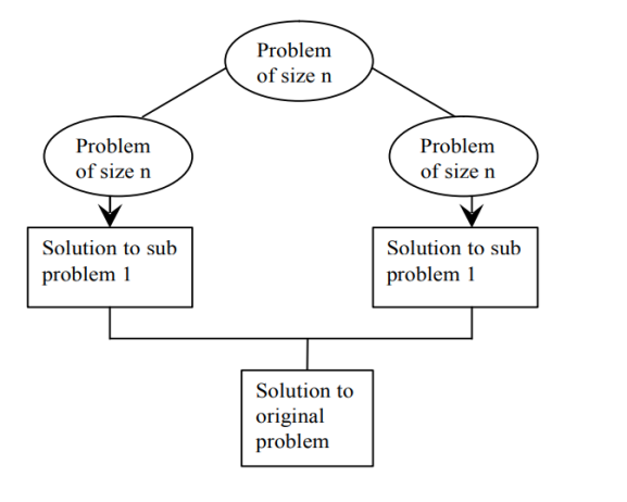
Divide & conquer is an efficient algorithm. It follows three steps:
● DIVIDE : divide problem into subproblems
● RECUR : Solve each sub problem recursively
● CONQUER : Combine all solutions of sub problem to get original solution
|
Fig 1: divide and conquer plan
Advantages of divide and conquer
● Divide to overcome conceptually challenging issues like Tower Of Hanoi , Divide & Conquering is a versatile instrument.
● Results with powerful algorithms
● The algorithms of Divide & Conquer are adapted to the execution of enemies in multi-processors Machines
● Results for algorithms that effectively use memory cache.
Disadvantages of divide and conquer
● Recursions are sluggish,
● It could be more complex than an iterative approach to a very simple problem.
Example: n numbers added etc.
General method
General divide and conquer recurrence :
It is possible to divide an example of size n into b instances of size n/b, with a need to resolve them. [a around 1, b > 1]. Assume that size n is a b-power. For running time T(n), the recurrence is as follows: T(n) = aT(n/b) + f(n) Where, f(n) - A function that accounts for the time spent on the problem being split into Smaller ones and to merge their alternatives. The order of growth of T(n) therefore depends on the values of the a & b constants and the order of growth of the f function (n). |
Master theorem
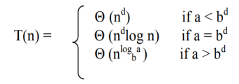
Theorem: If f(n) Є Θ (nd ) with d ≥ 0 in recurrence equation T(n) = aT(n/b) + f(n), then |
|
Example:
solve T(n) = 2T(n/2) + 1, using master theorem. Sol: Here, a = 2 b = 2 f(n) = Θ(1) d = 0 Therefore: a > bd i.e., 2 > 20 Case 3 of master theorem holds good. Therefore: T(n) Є Θ (nlog b a ) Є Θ (nlog 2 2 ) Є Θ (n) |
Key takeaways
- The strategy of divide and conquer implies that the given problem of size be divided Separate subproblems for n to k (1<k<=n).
- Typically, we write a control abstraction in the divide and conquer strategy that mirrors the way an algorithm would look.
- Control Abstraction is a procedure whose control flow is explicit but whose primary operations are specified by other processes that are left undefined with precise meanings.
The total idea of the coverage algorithm based on the chessboard coverage algorithm based on the divide and conquer strategy in the teaching materials is to first divide the chessboard into four sub-chess boards and then cover these four sub-chess boards, respectively.
The programme will first determine, for each sub-chessboard, whether the special pane is in that sub-chessboard. If the programme is in the sub-chessboard, it will recursively transfer the programme to cover that sub-chessboard, or else it will cover the adjacent panels with three additional sub-chessboards, and then recursively transfer the programme to cover that sub-chessboard.
Given condition:
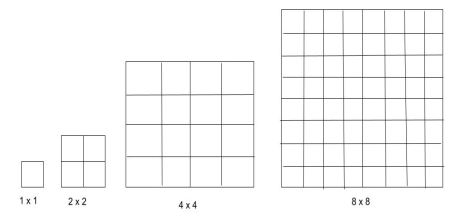
A chessboard is an n x n grid, where n =2k
|
Fig 2: n x n grid, chess board
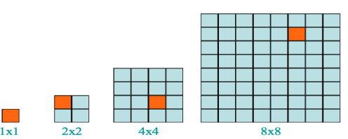
A chessboard that has one unavailable (defective) position is a defective chessboard.
|
Fig 3: defective chessboard
The issue is to use a triomino to tile (cover) all non defective cells.
A triomino is an object with a L shape that can cover three chessboard squares.
A triomino has four paths :
|
Fig 4: triomino
Objectives
Cover with L-shape tiles(trominoes) all the chessboard, excluding the faulty square.
Is it possible for this to be solved?
Ultimately, all non-defective squares can be sealed.
Let's take a look at how
● Since n x n and n= 2k are the size of the chessboard ● Complete number of squares = 2k x2k = 22k ● Number of squares that are not faulty = 22k-11k-11k ● Now, for K,22k-1, the value is divisible by 3. ● 22(1)-1 = 3 is divisible by 3 for E.g. K=1. ● K=2, 22(2) -1 =15 can be divided by 3. |
Defective chess board:
|
Fig 4: defective chess board
We don't have to put any L-shape tile in the first as the size of these chessboards shown here, 1x1 and 2x2, and the rest can be filled by just using 1 L-shaped tile.
Algorithm
- We just need to add a single tile to it for a 2x2 board with a faulty cell.
- In the centre, we will put an L-shape tile so that it does not cover the sub-square where it is already defective. The entire cell has a cell that is faulty.
- Repeat, recursively, this process until we have a 2x2 surface.
In general, a faulty 2k x 2k chessboard can be divided as—
2k - 1 x 2k - 1 | 2k -1 x 2k – 1 |
2k - 1 x 2k - 1 | 2k - 1 x 2k – 1 |
Analysis:
- Let n = 2k .
- Let t(k) be the time needed to tile a defective chessboard of 2k x 2k. Then, the,
|
- Here, c is a constant representation of time spent finding a triomino's appropriate location and rotating the triomino for a needed form.
t(k) = 4t(k-1) + c = 4[4t(k-2) + c] + c = 42 t(k-2) + 4c + c = 42 [4t(k-3) + c] + 4c + c = 43 t(k-3) + 42c + 4c + c = … = 4k t(0) + 4k-1c + 4k-2c + ... + 42c + 4c + c = 4k-1c + 4k-2c + ... + 42c + 4c + c = Θ(4k ) = Θ(number of triominoes placed)
|
Time complexity for defective chessboard problem
T(n) =4T(n/2) +C By Using Master Theorem, T(n) =a T(n/b) + Theta(n k log p n ), a>=1,b>1,k>=0 & p is the real number. a=4,b=2,k=0,p=0 a>b k => 4 >20 Case1: If a>bk , then T(n) =Theta(nlog b a). After putting the values of a and b the Time complexity for this problem = n2. |
Key takeaways
- The total idea of the coverage algorithm based on the chessboard coverage algorithm based on the divide and conquer strategy.
- first divide the chessboard into four sub-chessboards and then cover these four sub-chessboards, respectively.
● It is the searching method where we search an element in the given array
● Method starts with the middle element.
● if the key element is smaller than the middle element then it searches the key element into first half of the array ie. Left sub-array.
● If the key element is greater than the middle element then it searches into the second half of the array ie. Right sub-array.
This process continues until the key element is found. If there is no key element present in the given array then its searches fail.
Algorithm
Algorithms can be implemented as algorithms that are recursive or non-recursive.
ALGORITHM BinSrch ( A[0 … n-1], key) //implements non-recursive binary search //i/p: Array A in ascending order, key k //o/p: Returns position of the key matched else -1 l 0 r n-1 while l ≤ r do m ( l + r) / 2 if key = = A[m] return m else if key < A[m] r m-1 else l m+1 return -1 |
Analysis:
● Input size: Array size, n ● Basic operation: key comparison ● Depend on Best – Matching the key with the middle piece. Worst – Often a key is not identified or a key in the list. ● Let C(n) denote the number of times the fundamental operation is performed. Then one, then Cworst t(n)= Performance in worst case. Since the algorithm after each comparison is the issue is divided into half the size we have, Cworst (n) = Cworst (n/2) + 1 for n > 1 C(1) = 1 ● Using the master theorem to solve the recurrence equation, to give the number of when the search key is matched against an element in the list, we have: C(n) = C(n/2) + 1 a = 1 b = 2 f(n) = n0 ; d = 0 case 2 holds: C(n) = Θ (nd log n) = Θ (n0 log n) = Θ ( log n) |
Application:
- Guessing Number game
- Word Lists/Dictionary Quest, etc
Limitations :
- Interacting badly with the hierarchy of memory
- Allows the list to be sorted
- Because of the list element's random access, you need arrays instead of a linked list.
Advantages :
- Efficient on an incredibly broad list
- Iteratively/recursively applied can be
Example
Let us explain the following 9 elements of binary search:

The number of comparisons required to check for various components is as follows:
1. Searching for x = 101 low high mid 1 9 5 6 9 7 8 9 8 9 9 9 Found Number of comparisons: 4 2. Searching for x = 82 low high mid 1 9 5 6 9 7 8 9 8 Found Number of comparisons: 3 3. Searching for x = 42 low high mid 1 9 5 6 9 7 6 6 6 7 6 not Found Number of comparisons: 4 4. Searching for x = -14 low high mid 1 9 5 1 4 2 1 1 1 2 1 not Found Number of comparisons: 3 |
The number of element comparisons required to find each of the nine elements continues in this manner:
 No part needs seeking more than 4 comparisons. Summarizing the
Comparisons were required for all nine things to be identified and divided by 9, yielding 25/9 . On average, there are around 2.77 comparisons per effective quest.
Depending on the value of x, there are ten possible ways that an un-successful quest will end.
If x < a[1], a[1] < x < a[2], a[2] < x < a[3], a[5] < x < a[6], a[6] < x < a[7] or a[7] < x < a[8] The algorithm requires 3 comparisons of components to decide the 'x' This isn't present. Binsrch needs 4 part comparisons for all of the remaining choices. Thus, the average number of comparisons of elements for a failed search is: (3 + 3 + 3 + 4 + 4 + 3 + 3 + 3 + 4 + 4) / 10 = 34/10 =3.4 The time complexity for a successful search is O(log n) and for an unsuccessful search is Θ(log n). |
Key takeaways
- It is the searching method where we search an element in the given array
- if the key element is smaller than the middle element then it searches the key element into first half of the array ie. Left sub-array.
● Merge sort consisting two phases as divide and merge.
● In divide phase, each time it divides the given unsorted list into two sub list until each sub list get single element then sorts the elements.
● In merge phase, it merges all the solution of sub lists and find the original sorted list.
Features :
● Is an algorithm dependent on comparison?
● A stable algorithm is
● A fine example of the strategy of divide & conquer algorithm design
● John Von Neumann invented it.
Steps to solve the problem:
Step 1: if the length of the given array is 0 or 1 then it is already sorted, else follow step 2.
Step 2: split the given unsorted list into two half parts
Step 3: again divide the sub list into two parts until each sub list get single element
Step 4: As each sub list gets the single element compare all the elements with each other & swap in between the elements.
Step 5: merge the elements same as divide phase to get the sorted list
Algorithm:
ALGORITHM Mergesort ( A[0… n-1] ) //sorts array A by recursive mergesort //i/p: array A //o/p: sorted array A in ascending order if n > 1 copy A[0… (n/2 -1)] to B[0… (n/2 -1)] copy A[n/2… n -1)] to C[0… (n/2 -1)] Mergesort ( B[0… (n/2 -1)] ) Mergesort ( C[0… (n/2 -1)] ) Merge ( B, C, A ) ALGORITHM Merge ( B[0… p-1], C[0… q-1], A[0… p+q-1] ) //merges two sorted arrays into one sorted array //i/p: arrays B, C, both sorted //o/p: Sorted array A of elements from B & C I →0 j→0 k→0 while i < p and j < q do if B[i] ≤ C[j] A[k] →B[i] i→i + 1 else A[k] →C[j] j→j + 1 k→k + 1 if i == p copy C [ j… q-1 ] to A [ k… (p+q-1) ] else copy B [ i… p-1 ] to A [ k… (p+q-1) ]
|
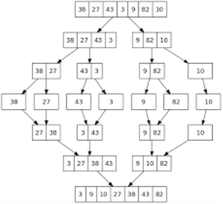
Example:
Apply merge sort for the following list of elements: 38, 27, 43, 3, 9, 82, 10
|
Analysis of merge sort:
All cases having same efficiency as: O (n log n) T (n) =T ( n / 2 ) + O ( n ) T (1) = 0 Space requirement: O (n) |
Advantages
● The number of comparisons carried out is almost ideal.
● Mergesort is never going to degrade to O (n2)
● It is applicable to files of any size.
Limitations
● Using extra memory O(n).
Key takeaways
- Merge sort consisting two phases as divide and merge.
- In divide phase, each time it divides the given unsorted list into two sub list until each sub list get single element then sorts the elements.
- In merge phase, it merges all the solution of sub lists and find the original sorted list.
● Quick sort algorithm works on the pivot element.
● Select the pivot element (partitioning element) first. Pivot element can be random number from given unsorted array.
● Sort the given array according to pivot as the smaller or equal to pivot comes into left array and greater than or equal to pivot comes into right array.
● Now select the next pivot to divide the elements and sort the sub arrays recursively.
Features
● Developed by C.A.R. Hoare
● Efficient algorithm
● NOT stable sort
● Significantly faster in practice, than other algorithms
Algorithm
ALGORITHM Quicksort (A[ l …r ]) //sorts by quick sort //i/p: A sub-array A[l..r] of A[0..n-1],defined by its left and right indices l and r //o/p: The sub-array A[l..r], sorted in ascending order if l < r Partition (A[l..r]) // s is a split position Quicksort(A[l..s-1]) Quicksort(A[s+1..r] ALGORITHM Partition (A[l ..r]) //Partitions a sub-array by using its first element as a pivot //i/p: A sub-array A[l..r] of A[0..n-1], defined by its left and right indices l and r (l <r) //o/p: A partition of A[l..r], with the split position returned as this function‘s value p→A[l] i→l j→r + 1; Repeat repeat i→i + 1 until A[i] >=p //left-right scan repeat j→j – 1 until A[j] < p //right-left scan if (i < j) //need to continue with the scan swap(A[i], a[j]) until i >= j //no need to scan swap(A[l], A[j]) return j |
Analysis of Quick Sort Algorithm
- Best case: The pivot which we choose will always be swapped into the exactly the middle of the list. And also consider pivot will have an equal number of elements both to its left and right sub arrays.
- Worst case: Assume that the pivot partition the list into two parts, so that one of the partition has no elements while the other has all the other elements.
- Average case: Assume that the pivot partition the list into two parts, so that one of the partition has no elements while the other has all the other elements.
Best Case | O (n log n) |
Worst Case | O (n2) |
Average Case | O (n log n ) |
Key takeaways
- Quick sort algorithm works on the pivot element.
- Select the pivot element (partitioning element) first. Pivot element can be a random number from a given unsorted array.
- Sort the given array according to pivot as the smaller or equal to pivot comes into the left array and greater than or equal to pivot comes into the right array.
References :
- Ellis Horowitz, Sartaj Sahni, Sanguthevar Rajasekaran: Fundamentals of Computer Algorithms, 2nd Edition, Universities Press, 2007.
- Thomas H. Cormen, Charles E. Leiserson, Ronal L. Rivest, Clifford Stein: Introduction to Algorithms, 3 rd Edition, PHI, 2010.
