Unit 4
Dynamic Programming
Dynamic programming (DP) is a general algorithm design technique for solving problems with overlapping subproblems. This technique was invented by American mathematician ― Richard Bellman in the 1950s.
● Dynamic programing solves the solutions of sub-problems
● Dynamic programing applies when sub-problem overlaps
● It solves each sub-problem just once and then saves answers in a table.
● Dynamic programming follows the basic principle of optimality.
● The principle of optimality says that problems can be solved by taking some decisions.
● In greedy methods we take decisions at one time only but in dynamic we take decisions at every stage.
Dynamic Programming is an algorithm design method that can be used when the solution to a problem may be viewed as the result of a sequence of decisions. Dynamic programming is a method that in general solves optimization problems that involve making a sequence of decisions by determining, for each decision, sub problems that can be solved in like fashion, such that an optimal solution of the original problem can be found from optimal solutions of sub problems.
An optimal policy has the property that whatever the initial state and initial decision are, the remaining decisions must constitute an optimal policy with regard to the state resulting from the first decision.
Dynamic Programming Properties :
- For smaller examples, an example is solved using the solutions.
- The solutions can be required many times for a smaller case, so store their results in a table.
- Each smaller instance is therefore resolved only once.
- To save time, extra space is used to
Rules of Dynamic Programming
- OPTIMAL SUBSTRUCTURE: Optimum solutions to sub-problems provide an optimal solution to a problem.
- OVERLAPPING SUBPROBLEMS: A recursive approach requires a small number of different sub-problems that are replicated several times.
- BOTTOM UP FASHION: Computes the solution in the final process in a bottom-up manner.
Three basic components of Dynamic Programming solution
The three basic components of the creation of a dynamic programming algorithm must be :
● A recurrence relation
● A tabular computation
● A backtracking procedure
Example Problems that can be solved using Dynamic Programming method
- Binomial coefficient computation
- Calculate the longest common subsequence
- Warshall's transitive closure algorithm.
- Floyd's all-pairs algorithm for the shortest paths.
- Some instances of difficult discrete optimization issues, such as the dilemma of knapsack and travelling salesperson.
Key takeaways
- Dynamic programming (DP) is a general algorithm design technique for solving problems with overlapping subproblems.
- Dynamic Programming is an algorithm design method that can be used when the solution to a problem may be viewed as the result of a sequence of decisions.
● Warshal’s algorithm constructs transitive closure of given directed graph.
● In directed graph there are n vertices.
● Warshal’s construct the transitive closure through series of matrices R0,R1,R2,….Rn and matrices order will be n*n.
● Rn become required transitive closure.
● Vertices are numbered from 1 to n.
● So the closure matrices series start from R0 then equation become
● R k[i,j]=R (k-1) [i,j]
Algorithm:
Algorithm Warshall(A[1..n, 1..n]) // Computes transitive closure matrix // Input: Adjacency matrix A // Output: Transitive closure matrix R R(0) A for k→1 to n do for i→ 1 to n do for j→ 1 to n do R(k)[i, j] → R(k-1)[i, j] OR (R(k-1)[i, k] AND R(k-1)[k, j] ) return R(n) |
Example:
|
Now, R(1) [i.j].R(0)[i,j] or (R(0)[i,1] & R(0) [1,j]) step 1 :- 1st row --> 2 (element at place 2 ) 1st col --> 3 (element at place 3 ) now R = {3,2} R (1) = |
|
step 2: 2nd row --> 3 2nd col --> 3,1 now R = { (1,3) , (3,3) } R2 = |
|
step 3: 3rd row --> 1,2,3,4 3rd col --> 1,2,3 R = { (1,1), (1,2), (1,3) , (1,4) (2,1), (2,2), (2,3), (2,4) (3,1), (3,2), (3,3), (3,4) } R2 = |
|
Efficiency:
● Time efficiency: Θ(n3 )
● Space efficiency: It needs extra space for separate matrices to record the algorithm's intermediate results.
Some Definitions:
● Directed Graphs: A graph with each edge directed is called a directed OR digraph graph.
● Adjacency matrix: The adjacency matrix of a directed graph A = {aij} is the Boolean matrix that has a directed graph.
● 1 - if from ith vertex to the jth vertex there is a directed edge.
● 0 - Otherwise
● Transitive Closure: It is possible to define the transitive closure of a directed graph with n vertices as the n-by-n matrix T={tij}, in which the elements in the ith row (1≤ I ≤ n) and the jth column (1 ≤ j ≤ n) are 1 if there is a nontrivial directed path (i.e. a positive length directed path) from the ith vertex to the jth vertex, otherwise tij is 0. The transitive closure provides data about a digraph with reach capability.
Key takeaways
● Warshall’s algorithm constructs transitive closure of given directed graph.
● In directed graph there are n vertices.
● A graph with each edge directed is called a directed OR digraph graph.
● Floyd's algorithm is used to find the shortest path from one node to all other nodes in the network.
● Hence it is also known as all pair shortest path algorithm.
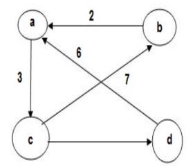
● Suppose there are four nodes such as A, B, C, D. If the source node is A then it finds the shortest path from A to all other nodes in the network as shown in figure given below.
|
Weighted graph: The weight of each edge is (associated numerical value). Depending on the set, edge weights can reflect costs, distance/lengths, capacities, etc. problem.
Algorithm:
Algorithm Floyd(W[1..n, 1..n]) // Implements Floyd‘s algorithm // Input: Weight matrix W // Output: Distance matrix of shortest paths‘ length D W for k → 1 to n do for i→ 1 to n do for j→ 1 to n do D [ i, j] → min { D [ i, j], D [ i, k] + D [ k, j] return D
|
Example:
|
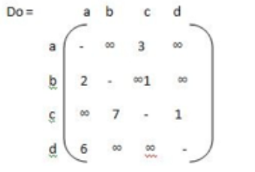
Step 1: construction of matrix. Do if i = j then wij = ‘ - ‘ else if i - - - > j = { c } else matrix ∞ |
|
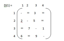
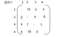
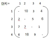
step 2:
k-1 k-1 k-1
W ij k = min ( Wij . Wik + Wkj )
|
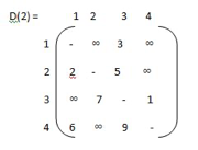
Step 3:
|
Key takeaways
- Floyd's algorithm is used to find the shortest path from one node to all other nodes in the network.
- The weight of each edge is (associated numerical value). Depending on the set, edge weights can reflect costs, distance/lengths, capacities, etc. problem.
● Weighted graph directed.
● Edges may have adverse costs.
● No loop whose price is < 0.0.
● Find the shortest path to each of the n vertices of the digraph from a given source vertex.
● Where there are negative-cost edges, Dijkstra's O(n2) single-source greedy algorithm does not work.
● The Bellman-Ford algorithm finds the bottom-up gap. It first finds certain distances in the route that have only one edge. Increase the length of the route after that to find all possible solutions.
Bellman - ford algorithm
● All-destinations of single-source shortest paths in
● Digraphs with cost-negative edges.
● Dynamic programming is used.
● Runs when adjacency matrices are used in O(n3) time.
● Runs in O(ne) time while using adjacency lists.
Algorithm
|
● To create the shortest path to vertex v from the source, decide on the maximum number of edges on the path and the vertex just before v.
● As there is no cycle in the digraph whose length is < 0,
● We can limit ourselves to the discovery of the shortest paths that are cycle-free (acyclic).
● A path that has no cycle has n-1 edges at most.
Cost function d
● Let d(v,k) (distk[v]) be the shortest path length from the source vertex to vertex v under the restriction that the path has edges of k at most.
● d(v,n-1) is the length of the shortest unrestricted path to vertex v from the source vertex.
● For each vertex v., we want to evaluate d(v,n-1).
Key takeaways
- The single source shortest path algorithm is also known Bellman-Ford algorithm is used to find minimum distance from source vertex to any other vertex.
- The main difference between this algorithm with Dijkstra’s algorithm is, in Dijkstra’s algorithm we cannot handle the negative weight, but here we can handle it easily.
Given a knapsack capacity c ∈ N and n objects A = {a0, . . . , an−1}, each having a nonnegative value v(ai) ∈ {x ∈ R : x ≥ 0} and a weight w(ai) ∈ N, the 0/1 knapsack problem (KS01) asks to pack the knapsack with a subset of objects from A, such that the sum of the weight of the chosen objects does not exceed the capacity c, and such that the sum of the values of the chosen objects is maximal. Let xi denote the binary decision variable of whether to include (i.e. xi = 1) object ai, or not (i.e. xi = 0). For brevity, we write vi for v(ai) and wi for w(ai). KS01 can also be formally stated as an integer LP problem: max z = |
|
s.t.
|
≤ c
xi ∈ {0, 1} ∀i ∈ {0, . . . , n − 1}.
The KS01 problem can be interpreted as a multistage decision problem in a straightforward manner. For each object ai, a decision xi has to be made whether to include ai, or not. Let the stage number i denote the index of the object currently under consideration and let w denote the space currently available in the knapsack.
The DP functional equation is
f(i,w) = 0 if i = −1 and 0 ≤ w ≤ c −∞ if i = −1 and w < 0 max {xivi + f(i − 1, w − xiwi)} if i ≥ 0 xi∈{0,1}
|
The goal is to compute f(n−1, c). The above DP functional equation can be slightly improved by introducing a decision set D = D(i,w) = _{0} if wi > w {0, 1} if wi ≤ w. that disallows infeasible decisions instead of punishing illegal states with a −∞ assignment. Replacing the static decision set {0, 1} used in (2.24) we get |
f(i,w) = 0 if i = −1 and 0 ≤ w ≤ c max {xivi + f(i − 1, w − xiwi)} if i ≥ 0 xi∈D
For instance, let c = 22, n = 3, A = (a0, a1, a2), (v0, v1, v2) = (25, 24, 15), and (w0, w1, w2) = (18, 15, 10). Then it is optimal to pick only object a0, in the final (i = 0) stage, and the optimal value of the knapsack is f(2, 22) = 25.
|
The integer knapsack problem, a variation of KS01 that allows integral decision variables xi, can be reduced to KS01, and vice versa.
● 0/1 knapsack problem is used to find the maximum profit from the items selected.
● 0/1 knapsack problem means we pick the item or not picking the item ie. We can't split the item.
● Item having the weight and the cost.
● Assume we are having many items then which item will give us more profit than we have to check first.
● First sort the value to weight in non-increasing order and then pick the item.
● Here I is row and j is column ● If (j<wt[i]) ● T[i][j]=T[i-1][j] ● Else ● { ● T[i][j]=max{val[i]+T[i-1][j-wt[i]] ● or ● {T[i-1][j] ● Here total weight =7 |
value | weight | 0 | 1 | 2 | 3 | 4 | 5 | 6 | 7 |
1 | 1 | 0 | 1 | 1 | 1 | 1 | 1 | 1 | 1 |
4 | 3 | 0 | 1 | 1 | 4 | 5 | 5 | 5 | 5 |
5 | 4 | 0 | 1 | 1 | 4 | 5 | 6 | 6 | 9 |
7 | 5 | 0 | 1 | 1 | 4 | 5 | 7 | 8 | 9 |
Key takeaways
- 0/1 knapsack problem is used to find the maximum profit from the items selected.
- 0/1 knapsack problem means we pick the item or not picking the item ie. We can't split the item.
The Traveling Salesman Problem (TSP) is a deceptively simple combinatorial problem. It can be stated very simply:
A salesman spends his time visiting n cities (or nodes) cyclically. In one tour he visits each city just once, and finishes up where he started. In what order should he visit them to minimize the distance travelled?
Many TSP's are symmetric that is, for any two cities A and B, the distance from A to B is the same as that from B to A. In this case you will get exactly the same tour length if you reverse the order in which they are visited so there is no need to distinguish between a tour and its reverse, and you can leave off the arrows on the tour diagram.
If there are only 2 cities then the problem is trivial, since only one tour is possible. For the symmetric case a 3 city TSP is also trivial. If all links are present then there are (n1)! Different tours for an n city asymmetric TSP. To see why this is so, pick any city as the first then there are n1 choices for the second city visited, n2 choices for the third, and so on.
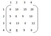
For the symmetric case there are half as many distinct solutions (n1)!/ 2 for an n city TSP. In either case the number of solutions becomes extremely large for large n, so that an exhaustive search is impractical. Given n cities and the distances dij between any two of them, we wish to find the shortest tour going through all cities and back to the starting city.
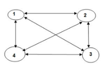
Usually the TSP is given as a G = (V,D) where V = {1, 2, . . . , n} is the set of cities, and D is the adjacency distance matrix, with ∀i, ∀jЄ V, i ≠ j, di,j > 0, the problem is to find the tour with minimal distance weight, that starting in 1 goes through all n cities and returns to 1.
The TSP is a well-known and difficult problem, that can be solved in O(n!) ~ O(nne-n) steps.
Characterization of the optimal solution
Given S ⊆ V with 1 ∈ S and given j ≠1, j ∈ S, let C(S, j) be the shortest path that starting at 1, visits all nodes in S and ends at j.
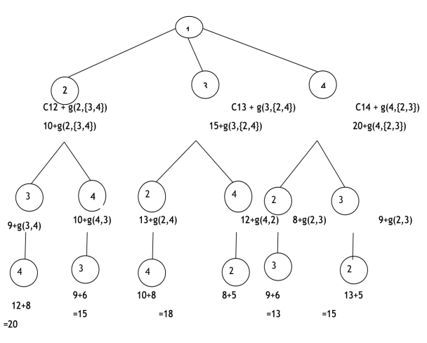
Notice: • If |S| = 2, then C(S, k) = d1,k for k = 2, 3, . . . , n • If |S| > 2, then C(S, k) = the optimal tour from 1 to m, +dm,k, ∃m ∈ S − {k} Recursive definition of the optimal solution C(S, k) = d1, m if S = {1, k} min m≠k, m∈S[C(S − {k},m) + d(m, k)] otherwise ● In travelling salesman problem start with source node travel all the nodes once and come back to the starting node and which path gives the minimum cost for travelling that becomes the optimal solution for travelling salesman problem. ● Formula: ● G(i,s)=min{Cik+ G( k, S- { k } )} TSP Algorithm. g (i,s) = min kϵs [Cik + g ( K , S – {K})]
|
Example:
|
|
|
|
g ( 1, { 2,3,4})
= min kϵ{2,3,4} { C 1k , g (K,{2,3,4}-{k})}
|
g(3,Φ)=6
g(4,Φ)=8
g(2,{3})=15
g(2,{4})=18
g(3,{2})=18
g(3,{4})=20
g(4,{2})=13
g(4,{3})=15
g(2,{3,4})=25
g(3,{2,4})=25
g(4,{3,2})=23
g(1,{2,3,4})=35
So the minimum optimal cost value from source node 1 to all other nodes is 35.
Key takeaways
- The Traveling Salesman Problem (TSP) is a deceptively simple combinatorial problem.
- In travelling salesman problem start with source node travel all the nodes once and come back to the starting node and which path gives the minimum cost for travelling that becomes the optimal solution for travelling salesman problem.
References
- Anany Levitin: Introduction to The Design & Analysis of Algorithms, 2nd Edition, Pearson Education, 2007.
2. Thomas H. Cormen, Charles E. Leiserson, Ronal L. Rivest, Clifford Stein: Introduction to Algorithms, 3rd Edition, PHI, 2010.


