Lower bound: an estimation of the minimum amount of work necessary to solve a particular issue.
Examples:
● The number of comparisons required in a set of n numbers to find the largest element.
● Number of comparisons needed to sort the n-size array.
● Number of comparisons required in a sorted array to check.
● The number of multiplications needed to multiply two matrices n-by-n the lower limit may be
– an exact count
– an efficiency class (Ω)
● Tight lower bound: an algorithm of the same efficacy as the lower bound exists
● Problem Lower bound Tightness sorting Ω(nlog n) yes searching in a sorted array Ω(log n) yes element uniqueness Ω(nlog n) yes n-digit integer multiplication Ω(n) unknown multiplication of n-by-n matrices Ω(n2) unknown
|
Methods for Establishing Lower Bounds
● Trivial lower bounds
● Information-theoretic arguments (decision trees)
● Adversary arguments
● Problem reduction
6.1.1 Trivial Lower Bounds:
The easiest way to get a lower-bound class is to count the number of items that need to be processed in the problem's input and the number of output items that need to be generated. Since every algorithm must at least "read" all the items that all its outputs need to be processed and "written," such a count yields a trivial lower bound.
Any algorithm for producing all permutations of n different objects, for example, must be in (n!) because the output size is n!. And this bond is strong since successful permutation generation algorithms spend constant time on each of them except the initial one.
Examples
• finding max element
• polynomial evaluation
• sorting
• element uniqueness
• computing the product of two n-by-n matrices
Conclusions
• may and may not be useful
• be careful in deciding how many elements must be processed
6.1.2 Information-Theoretic Arguments:
While the above approach takes into account the size of the output of a problem, the information-theoretical approach attempts to define a lower bound on the basis of the amount of information it has to generate.
As an example, consider the well-known game of deducting a positive integer between 1 and n chosen by someone by asking questions with yes/no answers from that person. Log2 n, the number of bits required to determine a specific number among the n possibilities, will calculate the amount of uncertainty that any algorithm that solves this issue has to solve.
We may think of each question (or, to be more precise, an answer to each question) as giving at most 1 bit of information about the performance of the algorithm, i.e. the number chosen. As a consequence, every such algorithm will require at least log2 n such steps until, in the worst case, it can evaluate its output.
Because of its relation to knowledge theory, the approach we just exploited is called the information-theoretical claim. For many problems involving comparisons, including sorting and searching, it has proved to be very useful for finding the so-called information-theoretical lower limits. Via the mechanism of decision trees, its underlying definition can be realised even more precisely.
6.1.3 Adversary Arguments:
Let us revisit the same "guessing" game used to apply the concept of an information-theoretical claim to a number. We can prove that in its worst case, any algorithm that solves this problem must ask at least log2 n questions by playing the function of an aggressive adversary who wants to ask as many questions as possible from an algorithm.
The opponent begins by considering each of the numbers between 1 and n as being theoretically chosen. (As far as the game is concerned, this is cheating, of course, but not as a way to prove our assertion.) The opponent gives an answer after each question that leaves him with the largest set of numbers compatible with this and all the answers previously given.
This method leaves him with at least half the numbers that he had before his last answer. If an algorithm stops before the set's size is reduced to 1, the opponent will show a number that may be a valid input that the algorithm has not defined. Now it is a simple technical matter to demonstrate that to shrink an n-element set to a one-element set by halving and rounding up the size of the remaining set, one requires log2n iterations. Therefore, in the worst case, every algorithm needs to ask at least log2n questions.
6.1.4 Problem Reduction:
There, by reducing it to another Q problem solvable with a proven algorithm, we discussed having an algorithm for problem P. For seeking a lower limit, a similar reduction concept can be used. We need to reduce Q to P (not P to Q!) to prove that problem P is at least as difficult as another problem Q with a known lower bound. In other words, we can prove that it is possible to convert an arbitrary instance of problem Q (in a relatively efficient way) to an instance of problem P, such that any algorithm solving P will also solve Q. A lower bound for Q will then be a lower bound for P.
Key takeaways
- Lower bound an estimation of the minimum amount of work necessary to solve a particular issue.
Many important algorithms work by comparing elements of their inputs, especially those for sorting and searching. With a system called a decision tree, we may research the efficiency of such algorithms.
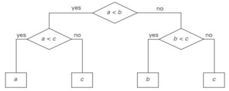
The decision tree of the algorithm for finding at least three numbers, each internal node of the binary decision tree, is a key comparison of the node, e.g. k < k . The left subtree of the node includes details about subsequent comparisons made if k < k, and the right subtree for k > k does the same. On some input of size n, each leaf represents a potential result of the algorithm's run.
Note that the number of leaves can be greater than the number of results since, by a different chain of comparisons, the same outcome can be obtained for certain algorithms.
The number of leaves must be at least as high as the number of potential outcomes, a significant point. The work of the algorithm on a particular input of size n can be traced in its decision tree by a path from the root to a leaf, and the number of comparisons made on such a run by the algorithm is equal to the length of this path.
Hence, in the worst case, the number of comparisons equals the height of the decision tree of the algorithm.
|
Fig 1: decision tree
Decision tree for sorting
• Number of leaves (outcomes) ≥ n!
• Height of a binary tree with n! leaves ≥ log2n!
• Minimum number of comparisons in the worst case ≥ log2n! for any comparison-based sorting algorithm
• log2n! ≈ n log2n
• This lower bound is tight (e.g. mergesort)
|
Fig 2: decision tree for three elements
Decision tree for searching a sorted array
• Number of leaves (outcomes) = n + n+1 = 2n+1 • Height of ternary tree with 2n+1 leaves ≥ log3 (2n+1) • This lower bound is NOT tight (the number of worst-case comparisons for binary search is log2 (n+1), and log3 (2n+1) ≤ log2 (n+1)) |
|
Fig 3: ternary decision tree for binary search
Key takeaways
- With a system called a decision tree, we may research the efficiency of such algorithms.
- The decision tree of the algorithm for finding at least three numbers, each internal node of the binary decision tree, is a key comparison of the node.
● The P class solves the problem of deterministic computation.
● P class is used to solve the problems that are solvable in polynomial run time.
● The problem belongs to class P if it’s easy to find a solution for the problem.
● These problems can be solved by the worst case in O(nK) where k is constant.
● The problems which are solved by P class that are known as tractable problems and others are known as intractable or super polynomial.
● If polynomial time is P(n) then the algorithm can solve in time O (P(n)) with input size n.
● The advantage of the class of polynomial time algorithms is that all reasonable deterministic single processor models of computation can be simulated on each other with at most polynomial slow-d.
● The NP class solves the problem of non-deterministic computation.
● The problem belongs to NP, if it’s easy to check a solution that may have been very tedious to find.
● It solves the problem which is verifiable by polynomial time.
● It is the class of decision problems.
● For using this class, it is easy to check the correctness of the claimed answer even if it has extra information added in it.
● Hence it is used to verify the solution is correct, not for finding the solution.
● If there is a problem in this class then it can be solved by exhaustive search in exponential time.
● NP complete class is used to solve the problems of no polynomial time algorithm.
● If a polynomial time algorithm exists for any of these problems, all problems in NP would be polynomial time solvable. These problems are called NP-complete.
● The phenomenon of NP-completeness is important for both theoretical and practical reasons.
● Following are the no polynomial run time algorithm:
- Hamiltonian cycles
- Optimal graph coloring
- Travelling salesman problem
- Finding the longest path in a graph, etc.
Application of NP complete class
- Clique
● A clique is a complete sub graph which is made by given undirected graph.
● All the vertices are connected to each other i.e.one vertex of undirected graph is connected to all other vertices in graph.
● There is the computational problem in clique where we can find the maximum clique of graph this known as max clique.
● Max clique is used in many real world problems and in many application.
● Assume a social networking where peoples are the vertices and they all are connected to each other via mutual acquaintance that becomes edges in graph.
● In the above example clique represents a subset of people who know each other.
● We can find max clique by taking one system which inspect all subsets.
● But the brute force search is too time consuming for a network which has more than a few dozen vertices present in the graph.
Example:
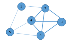
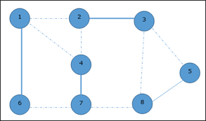
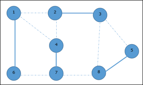
● Let's take an example where 1, 2, 3, 4, 5, 6 are the vertices that are connected to each other in an undirected graph.
● Here subgraph contains 2,3,4,6 vertices which form a complete graph.
● Therefore, subgraph is a clique.
● As this is a complete subgraph of a given graph. So it’s a 4-clique.
|
Fig 4: Analysis of Clique Algorithm
● Non deterministic algorithm uses max clique algorithm to solve problem.
● In this algorithm we first find all the vertices in the given graph.
● Then we check the graph is complete or not i.e. all vertices should form a complete graph.
● The no polynomial time deterministic algorithm is used to solve this problem which is known as NP complete.
2. Vertex Cover
● A vertex-cover of an undirected graph G = (V, E) is a subset of vertices V' ⊆ V such that if edge (u, v) is an edge of G, then either u in V or v in V' or both.
● In given undirected graph we need to find maximum size of vertex cover.
● It is the optimization version of NP complete problem.
● It is easy to find vertex cover.
Example:
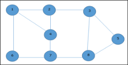
Given graph with set of edges are
{(1,6),(1,2),(1,4),(2,3),(2,4),(6,7),(4,7),(7,8),(3,8),(3,5),(8,5)}
|
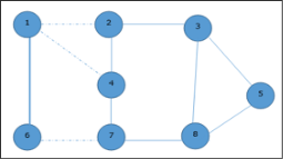
Now, start by selecting an edge (1, 6).
Eliminate all the edges, which are either incident to vertex 1 or 6 and we add edge (1, 6) to cover.
|
In the next step, we have chosen another edge (2, 3) at random
|
Now we select another edge (4, 7).
|
We select another edge (8, 5).
|
Hence, the vertex cover of this graph is {1, 2, 4, 5}.
Analysis of Vertex Cover Algorithm
● In this algorithm, by using adjacency list to represent E it is easy to see the running time of this algorithm is O (V+E).
Steps for proving a problem as NP-complete
First, try to prove it to be NP-hard, by :-
- Finding a related problem which is already found to be NP-hard (choosing such a suitable "source" problem close to your "target" problem, for the purpose of developing poly-trans, is the most difficult step), and then
- Developing a truth-preserving polynomial problem-transformation from that source problem to your target problem.
Significance: if anyone finds a poly algorithm for your “target” problem, then by using your poly-trans algorithm one would be able to solve that “source” NP-hard problem in poly-time, or in other words P would be = NP.
Second, try to prove that the given problem is in NP-class: by developing a polynomial algorithm for checking any "certificate" of any problem-instance.
The class P is the set of decision problems that can be solved in polynomial time.
P = {L | L ⊆ {0, 1}* and there exists an algorithm A that decides L in polynomial time}.
The branch of computer science concerned with algorithms for solving mathematical problems is generally defined as numerical analysis. This definition includes a major clarification: the problems in question are "continuous" mathematics problems, solving equations and equation systems, evaluating functions such as sin x and ln x, computing integrals, and so on, as opposed to discrete mathematics problems dealing with structures such as graphs, trees, permutations, and combinations.
Our interest in effective algorithms for mathematical problems stems from the fact that these problems occur both in the natural and social sciences as models of several real-life phenomena.
In fact, the main area of research, study and application of computer science used to be numerical analysis. The relative importance of numerical analysis has decreased in the last 30 years with the rapid proliferation of computers in business and everyday-life applications, which primarily deal with storage and retrieval of information.
However, it continues to expand its applications, enhanced by the power of modern computers, in all areas of fundamental research and technology. Thus, wherever one’s interests lie in the wide world of modern computing, it is important to have at least some understanding of the special challenges posed by continuous mathematical problems.
The job of explaining in mathematical terms a real-life phenomenon. Assuming this has already been done, what are the key hurdles we face to solving a mathematical problem?
The first big challenge is the fact that it is not possible to precisely solve most numerical analysis issues. They have to be solved roughly, and this is generally achieved by replacing a finite approximation with an infinite object.
For example, by approximating its infinite Taylor series around x = 0 by a finite sum of its first terms, called the nth-degree Taylor polynomial, the value of ex at a given point x can be computed:
|
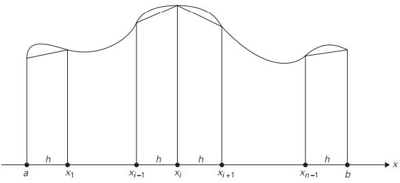
To give another example, as in the composite trapezoidal rule that you might recall from your calculus class, the definite integral of a function can be approximated by a finite weighted sum of its values:
where h = (b − a)/n, xi = a + ih for i = 0, 1, . . . , n
|
Truncation errors are considered the errors of such approximations. Estimating the magnitudes of truncation errors is one of the main tasks of numerical analysis. Typically, this is achieved through the use of calculus methods, from elementary to very advanced.
|
Fig 5: composite trapezoidal rule
Key takeaways
- The branch of computer science concerned with algorithms for solving mathematical problems is generally defined as numerical analysis.
- Our interest in effective algorithms for mathematical problems stems from the fact that these problems occur both in the natural and social sciences as models of several real-life phenomena.
- In fact, the main area of research, study and application of computer science used to be numerical analysis.
References
- Ellis Horowitz, Sartaj Sahni, Sanguthevar Rajasekaran: Fundamentals of Computer Algorithms, 2nd Edition, Universities Press, 2007.
- Thomas H. Cormen, Charles E. Leiserson, Ronal L. Rivest, Clifford Stein: Introduction to Algorithms, 3rd Edition, PHI, 2010.
