Unit 7
Coping with limitations of Algorithmic Power
● It is a general algorithmic technique.
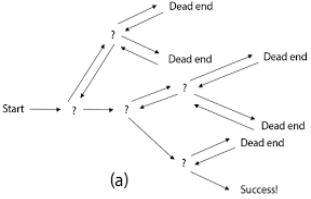
● Backtracking algorithm is used to solve a problem recursively to get a solution incrementally.
● It is used to solve problems when the sequence of objects is chosen from a specified set so that the sequence can satisfy some criteria.
● Backtracking is the systematic method which helps to try out a sequence of decisions until you find out that solution.
● It starts with one smaller piece at a time, if its solution get fails to satisfy the constraint then it can be removed at any point of time.
● It searches for any possible combination in order to solve a computational problem.
|
Fig 1: a - backtracking
● Two constraints :
- Implicit constraint
- Explicit constraint
● Application:
- N-queen problem
- Sum of subset
- Graph coloring
- Hamilton problems
N-Queens Problem
● Let chess board having N*N cells.
● We need to place N queens in such a way that no queen is attacked by any other queen.
● The queen can attack horizontally, vertically and diagonally.So initially, we are having N*N unattacked cells where we can place the N queens.
Step 1: Place the first queen at a cell (i,j). Hence the unattacked cell is reduced and the number of queens to be placed is N−1.
Step 2: Place the second queen on an unattacked cell that will reduce the no. of unattacked cells and no. of queen to be placed become N-2.
The process continues until it satisfies the following condition.
The no. of unattacked cell become 0
The no of queens to be placed is not 0.
Step 3: As it satisfies the first condition given above then it’s over, we got a final solution.
But if the unattacked cells become 0, then we need to backtrack and remove the last placed queen from its current place and place it in another cell.
This process will be done recursively.
Example:
8-Queen problem
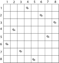
● The eight-queen problem is the problem of placing eight queens on an 8×8 chessboard such that none of them attack one another.
● The eight-queen puzzle has 92 distinct solutions.
● If a solution that differs only by symmetry operation of the board are counted as one puzzle has 12 unique solutions.
Formulation of problem:
● States: any arrangement of 8 queens on board
● Initial state: 0 queens on the board
● Successor function: add a queen on any square
● Goal state: unattacked 8 queens on the board
Steps to be perform:
- Place the first queen in the left upper corner of the table
- Save the attacked position
- Move to the next queen which can only placed on next line
- Search for a valid position. (unattacked position) If there is one go to step 8.
- There is not a valid position for a queen then delete it.
- Move to the previous queen
- Got to step 4
- Place it to the first valid position
- Save the attacked positions
- If the queen processed is the last stop otherwise go to step 3.
Algorithm:
putQueen(row) { For every position col on the same row If the position col is available Place the next queen in position col If(row<8) putQueen(row+1) else success remove the queen from positioncol } |
Key takeaways
- Backtracking algorithm is used to solve a problem recursively to get a solution incrementally.
- It is a general algorithmic technique.
- It searches for any possible combination in order to solve a computational problem.
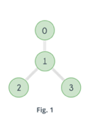
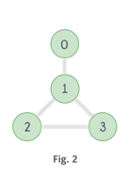
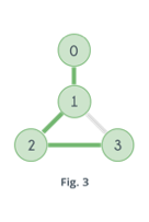
The Hamilton path is the path from first vertex to last vertex which visits each vertex exactly once in an undirected or directed graph.
Hamilton cycle is the circuit in which there is an edge from the last vertex to the first vertex.
In this problem we can determine whether a graph contains a Hamilton cycle or not. If the cycle presents then it prints the cycle.
|
|
|
|
Fig 2: Hamilton cycle
Key takeaways
- Hamilton cycle is the circuit in which there is an edge from the last vertex to the first vertex.
- In this problem we can determine whether a graph contains a Hamilton cycle or not. If the cycle presents then it prints the cycle.
● In this problem there is a given set with integer numbers and also some other values provided. We have to find a subset of a given set whose sum is the same as the given sum value.
|
● Here backtracking is used for trying to select a valid subset when a number is not valid. We will backtrack to get the previous subset and add another number to get a solution.
● In the backtracking algorithm we need to explore the nodes along the breadth and depth of the tree.
● Generating nodes along breadth is controlled by loop and nodes along the depth are generated using recursion.
● This problem is based on a post order traversal method.
● Following are the steps to solve the problem:
Step 1: start with an empty set
Step 2: Add element from given list to the set
Step 3: If the set is having sum M then stop with that subset as solution
Step 4: if the set is not feasible then backtracks until we find the solution.
Step 5: If the set is feasible and sum of subset < M then go to step 2
Step 6: if we have visited all numbers given in the set without finding a suitable solution and if no backtrack is possible then stop.
Example:
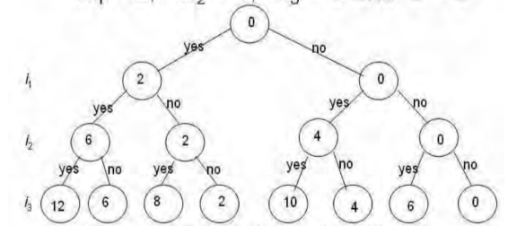
Given set of numbers= {1,3,2,4} Find subsets with sum=3 Step 1: consider an empty set{ } Add 1 into empty set { 1 } (sum=1,1<3) Add 3 into set {1,3} (sum=4,4>3,backtrack) Remove 3 from subset { 1 } Add 2 into set { 1,2 } (sum=3,3=3,found solution) We remove 2 and check all elements have been considered. Solution: { } {1} {1, 3}(backtrack) {1} {1,2 }(found) {1}(end) ● Problem: Considering the n positive integer w1,... Wn, and S with a positive integer. Select all of the w1 subsets, ... Wn to S for that number. ● For example : N=3, w1=2, w2=4, w3=6, and S=6 ● Solutions: {2,4} and {6}, respectively, ● We will assume a space tree with a binary state. ● Nodes at depth 1 are intended to include (yes, no) item 1, and nodes at depth 2 are intended for item 2, etc. ● Wi contains the left branch, and wi is absent from the right branch. ● The nodes hold the sum of the weights so far included.
|
Sum of subset Problem: State SpaceTree for 3 items
W1 = 2, W2 = 4, W3 = 6 & S = 6
|
Fig 3: example of subset problem
Sum of the included integers is stored at the node.
Backtracking Solution to Sum of Subset
● Definition: If it does not lead to a feasible (or optimal) solution, we call a node non-promising, otherwise it is promising.
● Main motivation: Backtracking includes doing a state space tree DFS, testing if each node is promising and if the node is not promising to backtrack to the parent of the node.
● The state space tree is called the pruned state space tree, consisting only of extended nodes.
● For the sum of subsets, for example, the following slide shows the pruned state space tree
● Just 15 nodes in the pruned state space tree exist.
● The 31 nodes of the complete state space tree are.
Key takeaways
- Here backtracking is used for trying to select a valid subset when a number is not valid.
- We will backtrack to get the previous subset and add another number to get a solution.
- This problem is based on a post order traversal method.
● Without an exhaustive search in the typical case, this technique can be used to solve optimization issues.
● 2 Methodologies:
- A branch-generating mechanism when searching the solution space
- A mechanism for generating a connection so that many brakes can be stopped
● In the average example, it is successful since several divisions can be terminated very early.
● Although it is generally very effective, in the worst case, a very large tree will be produced.
● In the average case, many NP-hard problems can be solved effectively by Branch & Bound; however, the worst-case time complexity is still exponential.
Assignment problem
● Management needs to assign - personnel to jobs, - jobs to machines, - machines to job locations, or - salespeople to territories in many business situations.
● Consider the scenario of n jobs being allocated to n machines.
● If a work I (=1,2,....,n) is allocated to machine j (=1,2, .....n) at the expense of Cij.
● The goal is to assign the jobs to machines at the minimum total cost possible.
● A special case of the Transportation Model is this situation and it is known as the problem of assignment.
● Employment here is represented by sources and machines representing destinations.
● The supply available is 1 unit at each source, and the demand is 1 unit at each destination.
job | Machine | |||||
| 1 | 2 | . . . . . . | n | Source | |
1 | C11 | C12 | . . . . . . | C1n | 1 | |
2 | C21 | C22 | . . . . . . | C2n | 1 | |
– | . | . |
| . | – | |
– | . | . |
| . | – | |
– | . | . |
| . | – | |
n | Cn1 | Cn2 | . . . . . . | Cnn | 1 | |
Destination | 1 | 1 | 1 | . . . . . . | 1 |
|
It is possible to mathematically express the assignment model as follows:
Xij= 0, if the job j is not assigned to machine i
1, if the job j is assigned to machine i
Assignment analysis problem:
● Tiny electrical devices are developed by Ballston Electronics.
● Products on five different assembly lines (1,2,3,4,5) are manufactured.
● Products are transported from the assembly lines to one of the five different inspection areas (A, B, C, D, E) when production is completed.
● Transporting goods to five inspection areas from five assembly lines needs different times (in minutes).
|
The assignment of inspection areas to assembly lines is 1 to A, 2 to B, 3 to C, 4 to D, and 5 to E, as provided for in the current arrangement. This scheme requires 10+7+12+17+19=65 minutes for an individual.
● Management would like to decide if certain other assignments of production lines to inspection areas could result in lower costs.
● This is a common issue with assignments. N = 5 And each assembly line is allocated to each area of inspection.
● Such a problem would be easy to solve when n is 5, but when n is big, all possible alternative solutions are n! This is becoming a difficult issue.
● The problem of assignment can either be formulated as a linear programming model or it can be formulated as a model of transport.
● An algorithm known as the Hungarian Method, however, has proved to be a fast and successful way to solve such issues.
Assignment problem revisited:
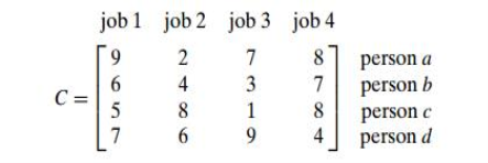
In every row of the cost matrix C, select one element so that:
● No two elements are selected in the same column,
● The number is reduced
Example:
|
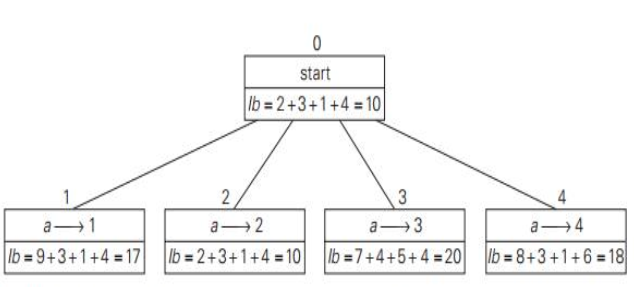
Lower bound: The overall cost of any solution to this issue would be at least :
2 + 3 + 1 + 4 (or 5 + 2 + 1 + 4)
Example: First two levels of the state-space tree
|
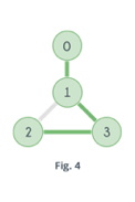
Fig 4: two level (0,1) of state space tree
|
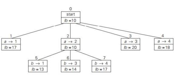
Fig 5: three level (0,1,2) of state space tree for assignment problem
|
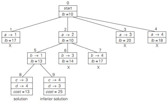
Fig 6: complete state space tree for assignment problem
Key takeaways
- Without an exhaustive search in the typical case, this technique can be used to solve optimization issues.
- A special case of the Transportation Model is this situation and it is known as the problem of assignment.
- Employment here is represented by sources and machines representing destinations.
● We are given n no. of objects with weights Wi and profit Pi where I varies from 1 to n and also a knapsack with capacity M
● The problem is, we have to fill the bag with the help of n objects and the resulting profit has to be maximum.
● This problem is similar to the ordinary knapsack problem but we may not take a function of an object.
Example:
Profit | 10 | 10 | 12 | 18 |
weight | 2 | 4 | 6 | 9 |
In this problem we find upper bound and lower bound for each node.
● To calculate upper bound,
Place first item in knapsack calculate remaining weight ie. 15-2=13 Place next item in knapsack and remaining weight is 13-4=9 Place next item in knapsack and remaining weight is 9-6=3 Fraction is not allowed in calculation of upper bound in knapsack hence next item cannot be placed in the knapsack. Profit=p1+p2+p3=10+10+12=32 ie. Upper bound |
● To calculate lower bound,
Fraction is allowed in calculation of lower bound in knapsack hence the next item can be placed in the knapsack.
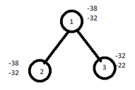
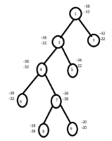
Lower bound=10+10+12+(3/9*18)=32+6=38 Knapsack is a maximization problem but branch and bound can be applied on minimization problems. Hence to convert maximization problem into minimization we have to take negative sign for upper bound and lower bound. Therefore, upper bound (U)=-32 Lower bound(L)=-38 We choose the path which has minimized difference of upper bound and lower bound. If the difference is equal then choose the path by comparing upper bound and discard node with maximize upper node. Now calculate upper and lower bound for remaining nodes. For node 2, U=10+10+12=32 ≈ -32 L=10+10+12+(3/9*18)=32+6=38 ≈ -38 For node 3, U=10+12=22 L=10+12+(5/9*18)=32 ≈ -32 |
|
Calculate the difference of upper bound and lower bound for 2,3.
For node 2, U-L=-32+38=6
For node 3, U-L=-22+32=10
|
Select node 2 since it has a minimum difference value of 6.
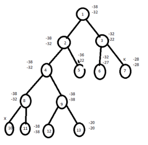
Similarly continues the process, Calculate difference of lower and upper bound of nodes 8 ,9. For node 8,U-L=-38+38=0 For node 9,U-L=-20+20=0 Here the difference is the same hence compare the upper bound of node 8 and 9. Discard the node with maximum upper bound. Consider the path from 1→ 2→4→7→8 The solution for 0/1 knapsack problem is (1,1,0,1) Maximum profit= ∑PiXi = 10*1+10*1+12*0+18*1=10+10+18=38 FIFO branch and bound solution Let's assume the above example in this problem. Initially node 1 is E node and the queue of live nodes are empty. Here U=-32 hence node 2 and 3 are generated as children of node 1 and added to the queue. The value of the upper bound remains unchanged. Now node 2 becomes E node and its children are added to the queue. Next node 3 is expanded and its children are generated. Node 6 is also added to the queue. Node 7 is killed as L(7)>U. |
Next node 4 is expanded. Continue the process until it gets the solution.
|
Key takeaways
- This problem is similar to the ordinary knapsack problem but we may not take a function of an object.
- We are given n no. of objects with weights Wi and profit Pi where I vary from 1 to n and also a knapsack with capacity M
Steps to solve travelling salesman problem:
Step 1: reduce the given cost matrix in which every row and column is reduced. This can be done as follows:
Row Reduction:
● Take the minimum element from the first row, subtract it from all elements of the first row,next take the minimum element from the second row and subtract it from the second row. Similarly apply the same procedure for all rows.
● Find the sum of elements, which were subtracted from rows.
● Apply column reductions for the matrix obtained after row reduction.
Column reduction
● Take the minimum element from the first column, subtract it from all elements of the first column, next take the minimum element from the second column and subtract it from the second column. Similarly apply the same procedure for all columns.
● Find the sum of elements, which were subtracted from columns.
● Obtain the cumulative sum of row wise reduction and column wise reduction.
● Cumulative reduced sum=Row wise reduction sum + Column wise reduction sum.
● Associate the cumulative reduced sum to the starting state as lower bound and α as upper bound.
Step 2: Calculate the reduced cost matrix for every node.
● If path (i,j) is considered then change all entries in row i and column j of A to α.
● Set A(j,1) to α.
● Apply row reduction and column reduction except for rows and columns containing only α. Let r is the total amount subtracted to reduce the matrix.
● Find ĉ(S)= ĉ(R)+A(i,j)+r.
● Repeat step 2 until all nodes are visited
Example:
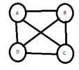
|
Given cost adjacency matrix
A B C D
A ∞ 4 6 2
B 7 ∞ 5 3
C 2 1 ∞ 9
D 8 7 2 ∞
LET stating node is A
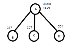
So upper bound= ∞
Row Reduction
∞ | 2 | 4 | 0 |
4 | ∞ | 2 | 0 |
1 | 0 | ∞ | 8 |
6 | 5 | 0 | ∞ |
1 | 0 | 0 | 0 |
Minimum value
∞ | 4 | 6 | 2 | 2 |
7 | ∞ | 5 | 3 | 3 |
2 | 1 | ∞ | 9 | 1 |
8 | 7 | 2 | ∞ | 2 |
 Minimum value
Minimum value of each row is 2,3,1,2
Total reduction = (2+3+1+2) + 1=9
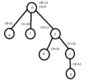
CA = 9
|
∞ | 2 | 4 | 0 |
3 | ∞ | 2 | 0 |
0 | 0 | ∞ | 8 |
5 | 5 | 0 | ∞ |
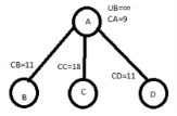
Let choose AB
So C[A,B] = 2
CA=9
PUT A ROW∞
B COLUMN∞
C[B,A] ∞
∞ | ∞ | ∞ | ∞ |
∞ | ∞ | 2 | 0 |
0 | ∞ | ∞ | 8 |
5 | ∞ | 0 | ∞ |
We get same column after row
column reduction.
Therefore reduction=0
Hence, CB=C[A,B]+CA+REDUCTION
=2+9+0
=11
Let choose AB
C[A,C]=4 AND CA=9
PUT A ROW∞
C COLUMN∞
C[C,A] ∞
∞ | ∞ | ∞ | ∞ |
3 | ∞ | ∞ | 0 |
∞ | 0 | ∞ | 8 |
5 | 5 | ∞ | ∞ |
We get column after row & column reduction.
Therefore reduction=5
∞ | ∞ | ∞ | ∞ |
3 | ∞ | ∞ | 0 |
∞ | 0 | ∞ | 8 |
0 | 0 | ∞ | ∞ |
So Cc=C[A,C]+CA+REDUCTION
=4+9+5=18
Lets choose AD
SO C[A,D]=0 & CA=9
PUT A ROW∞
D COLUMN∞
C[D,A] ∞
∞ | ∞ | ∞ | ∞ |
3 | ∞ | 2 | 0 |
0 | 0 | ∞ | 8 |
∞ | 5 | 0 | ∞ |
WE GET CAM AFTER row and
column reduction as,
reduction=2
∞ | ∞ | ∞ | ∞ |
1 | ∞ | 0 | ∞ |
0 | 0 | ∞ | ∞ |
∞ | 5 | 0 | ∞ |
So CD=C[A,D]+CA+REDUCTION=0+9+2=11
|
LET'S CHOOSE AD
SO REDUCTION MATRIX IS,
∞ | ∞ | ∞ | ∞ |
1 | ∞ | 0 | ∞ |
0 | 0 | ∞ | ∞ |
∞ | 5 | 0 | ∞ |
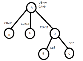
ENTERING NODE D.
|
LET CHOOSE ADB
C[D,B]=5 & CD=11
PUT D ROW∞
B COLUMN∞
C[B,D] ∞ & C[B,A] ∞
∞ | ∞ | ∞ | ∞ |
∞ | ∞ | 0 | ∞ |
0 | ∞ | ∞ | ∞ |
∞ | ∞ | ∞ | ∞ |
CAM AFTER REDUCTION IS SAME IE.
REDUCTION=0
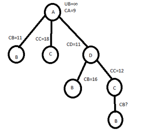
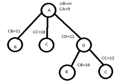
CB=5+11+0=16
LET CHOOSE ADC
C[D,C]=0 & CD=11
PUT D ROW∞
C COLUMN∞
C[C,D] ∞ & C[C,A] ∞
∞ | ∞ | ∞ | ∞ |
1 | ∞ | ∞ | ∞ |
∞ | 0 | ∞ | ∞ |
∞ | ∞ | ∞ | ∞ |
NOW REDUCTION = 1
∞ | ∞ | ∞ | ∞ |
0 | ∞ | ∞ | ∞ |
∞ | 0 | ∞ | ∞ |
∞ | ∞ | ∞ | ∞ |
CC=0+11+1=12
HENCE WE SELECT C, ADC
NOW WE EXPLORE NODE C
|
|
REDUCED MATRIX,
∞ | ∞ | ∞ | ∞ |
0 | ∞ | ∞ | ∞ |
∞ | 0 | ∞ | ∞ |
∞ | ∞ | ∞ | ∞ |
CHOOSE , ADCB
C[C,B]=0 & CC=0
PUT C ROW∞
B COLUMN∞
C[B,C] ∞ & C[C,A] ∞
∞ | ∞ | ∞ | ∞ |
∞ | ∞ | ∞ | ∞ |
∞ | ∞ | ∞ | ∞ |
∞ | ∞ | ∞ | ∞ |
NOW REDUCTION = 0
CB=0+12+0=12
|
PATH IS, ADCBA WITH COST 12.
Key takeaways
- Row reduction: Take the minimum element from the first row, subtract it from all elements of the first row, next take the minimum element from the second row and subtract it from the second row.
- Column reduction: Take the minimum element from the first column, subtract it from all elements of the first column, next take the minimum element from the second column and subtract it from the second column.
● A problem is in the class NPC if it is in NP and is as hard as any problem in NP.
● A problem is NP-hard if all problems in NP are polynomial time reducible to it, even though it may not be in NP itself.
● The problem in NP-Hard cannot be solved in polynomial time, until P = NP.
● If a problem is proved to be NPC, there is no need to waste time on trying to find an efficient algorithm for it.
● Instead, we can focus on design approximation algorithm.
● Following are the NP hard class problems:
- Circuit satisfiability problem
- Set cover
- Vertex cover
- Travelling salesman problem
● This is a traditional CS problem.
● A minimum weight tour of the cities is found according to a graph (cities) and weights on the edges (distances).
- Starting in a specific city
- Visit all other towns (exactly once each)
- Return to the city that starts
● It can not be done by brute force as this is exponential or worse in the worst case.
- So we're going to look at backtracking with pruning to make it run reasonably.
● Amount of time in most circumstances
● We are going to create our State Space by:
- Getting our children are all the prospective cities that we will go to next
- Getting the tree depth equal to the number of towns in the graph
● We must visit each town exactly once.
● So we have the following state space, given a completely linked set of 5 nodes,
- Just completed partially.
Example: Traveling Salesman Problem
Round up the result to the nearest integer if all the distances are integers:
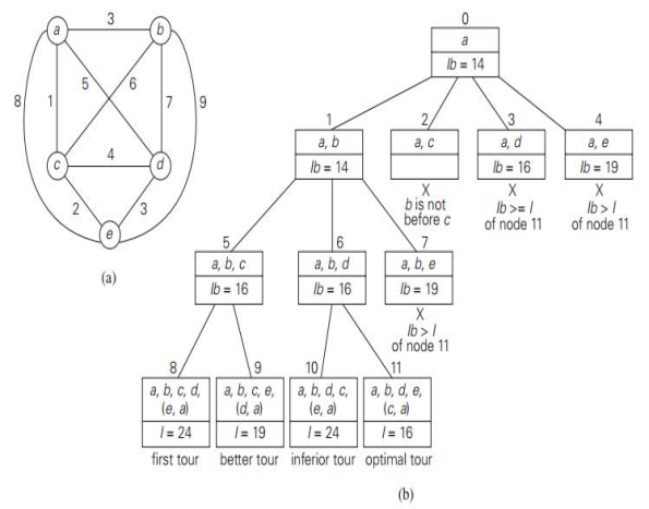
lb = [s/2] For instance, formula produces : lb = [ [(1+3) + (3+6) + (1+2) + (3+4) + (2+3)] / 2 ] = 14 By summing the lengths of the two shortest edges with each of the vertices, with the necessary inclusion of edges (a, d) and (d, a), we get the following lower bound: [ [ (1+5) + (3+6) + (1+2) + (3+5) + (2+3) ] /2 ] = 16. |
We now apply the branch-and-bound algorithm to find the shortest Hamiltonian circuit for the graph in the bounding function given by the formula.
|
Fig 7: (a) – weighted graph
(b) – state space tree
Key takeaways
- A minimum weight tour of the cities is found according to a graph (cities) and weights on the edges.
- It can not be done by brute force as this is exponential or worse in the worst case.
- We must visit each town exactly once.
Step 1: Order the elements in the order of relative values decreasing:
Step 2: Generate all subsets of k items or less for a given integer parameter k, 0 ≤ k ≤ n, and add the remaining items in decreasing order of their value to weight ratios for each of those that match the knapsack.
Step 3: Find the most valuable subset of the Phase 2 generated subsets and return it as the output of the algorithm.
Solving the problem of the knapsack by a branch-and-bound algorithm has a very unusual feature. Usually, internal nodes in a state-space tree do not identify a point in the search space of the problem, so some of the components of the solution remain undefined.
However, for the knapsack problem, every tree node represents a subset of the items given. After generating each new node in the tree, we can use this fact to update the details about the best subset seen so far.
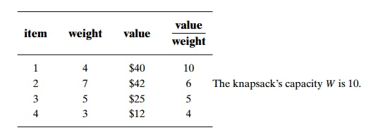
Let us apply the branch-and-bound algorithm as a particular example to the same instance of the knapsack problem we solved by exhaustive search. (In descending order of their value-to-weight ratios, though, we reorder the items.)
Example:
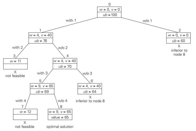
A easy way to measure the upper bound ub is to add the total value of the already selected items to v, the product of the knapsack's remaining capacity W-w and the best payoff per unit among the remaining items, which is vi+1/wi+1:
ub = v + (W - w) (vi+1 / wi+1) |
|
|
Fig 8: state space tree for B & B of knapsack problem
Key takeaways
- Solving the problem of the knapsack by a branch-and-bound algorithm has a very unusual feature.
- Usually, internal nodes in a state-space tree do not identify a point in the search space of the problem, so some of the components of the solution remain undefined.
References
- Ellis Horowitz, Sartaj Sahni, Sanguthevar Rajasekaran: Fundamentals of Computer Algorithms, 2nd Edition, Universities Press, 2007.
- R.C.T. Lee, S.S. Tseng, R.C. Chang & Y.T.Tsai: Introduction to the Design and Analysis of Algorithms A Strategic Approach, Tata McGraw Hill, 2005.
