UNIT-3
Complex Integration
|
In case of a complex function f(z) the path of the definite integral  can be along any curve from z = a to z = b.
In case the initial point and final point coincide so that c is a closed curve, then this integral called contour integral and is denoted by-
|

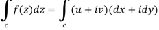
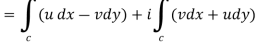
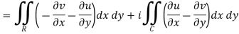
If f(z) = u(x, y) + iv(x, y), then since dz = dx + i dy
We have-
|

It shows that the evaluation of the line integral of a complex function can be reduced to the evaluation of two line integrals of real function.
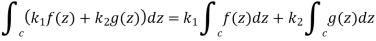
Properties of line integral-
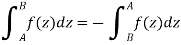
2. Sense reversal-
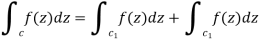
3. Partitioning of path-
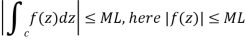
4. ML – inequality-
|


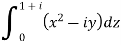
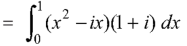
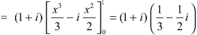
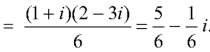
Example: Evaluate
|
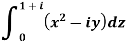
along the path y = x.
Sol.
Along the line y = x, dy = dx that dz = dx + i dy dz = dx + i dx = (1 + i) dx
On putting y = x and dz = (1 + i)dx
|
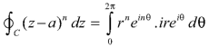
Example: Evaluate
|

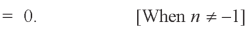
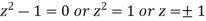
where c is the circle with center a and r. What is n = -1.
Sol.
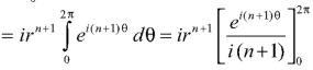
The equation of a circle C is |z - a| = r or z – a = Where dz =
Which is the required value. When n = -1
|


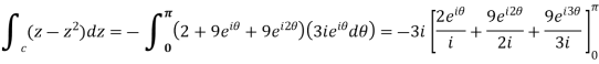
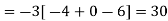
Example: Evaluate
|

where c is the upper half of the circle |z – 2| = 3.
Find the value of the integral if c is the lower half of the above circle.
Sol.
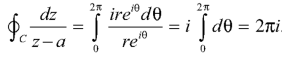
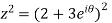
The equation of the circle is-
Or
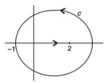
Now for the lower semi circle-
|


Key takeaways-
3. Sense reversal-
4. Partitioning of path-
5. ML – inequality-
|


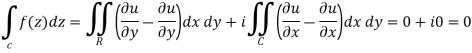
A function f(z) is analytic and its derivative f’(z) continuous at all points inside and on a closed curve c, then
|

Proof:
Suppose the region is R which is closed by curve c and let-
By using Green’s theorem-
Replace
So that-
|


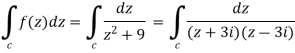
Example-1: Evaluate
|

Sol.
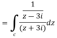
Here we have-
Hence the poles of f(z),
Note- put determine equal to zero to find the poles.
Here pole z = -3i lies in the given circle C. So that-
|


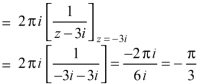
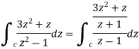
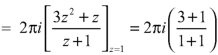
Example 2:
|


Sol.
= =
|
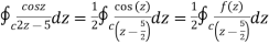


Example 3:
Solve the following by cauchy’s integral method:
|
Solution:
Given,
= = = |
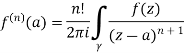
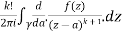
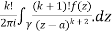
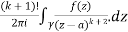
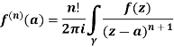
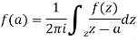
Cauchy’s integral formula-
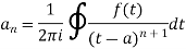
Cauchy’s integral formula can be defined as-
|

Where f(z) is analytic function within and on closed curve C, a is any point within C.
Example-1: Evaluate
|
by using Cauchy’s integral formula.
Here c is the circle |z - 2| = 1/2
Sol. it is given that-
Find its poles by equating denominator equals to zero.
There is one pole inside the circle, z = 2, So that-
Now by using Cauchy’s integral formula, we get-
|

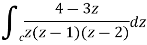
Example-2: Evaluate the integral given below by using Cauchy’s integral formula-
|
Sol.
Here we have-
Find its poles by equating denominator equals to zero.
We get-
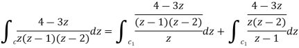
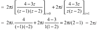
There are two poles in the circle- Z = 0 and z = 1 So that-
|

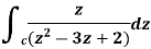
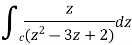
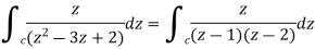
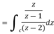
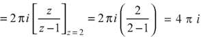
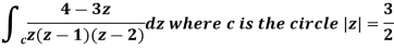
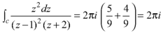
Example-3: Evaluate
|

Sol.
Here we have-
Find its poles by equating denominator equals to zero.
The given circle encloses a simple pole at z = 1. So that-
|


Key takeaways-
|

Taylor’s series-
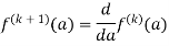
If f(z) is analytic inside a circle C with centre ‘a’ then for z inside C,
|

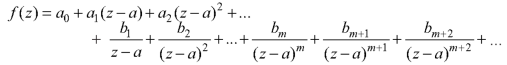
Laurent’s series-
If f(z) is analytic in the ring shaped region R bounded by two concentric circles C and  of radii ‘r’ and
  where r is greater and with centre at’a’, then for all z in R
Where
|

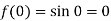
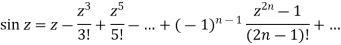
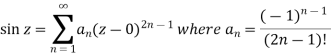
Example: Expand sin z in a Taylor’s series about z = 0.
Sol.
It is given that-
Now-
We know that, Taylor’s series-
So that
Hence
|


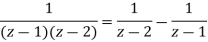
Example: Expand
f(z) = 1/ [(z - 1) (z - 2)] |
in the region |z| < 1.
Sol.
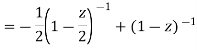
By using partial fractions-
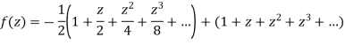
Now for |z|<1, both |z/2| and |z| are < 1, Hence we get from second equation-
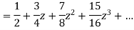
Which is a Taylor’s series. |
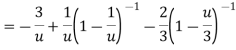
Example: Find the Laurent’s expansion of-
|
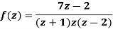
In the region 1 < z + 1< 3.
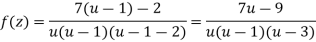
Sol.
Let z + 1 = u, we get-
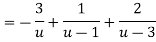
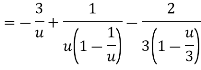
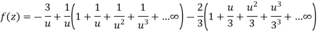
Here since 1 < u < 3 or 1/u < 1 and u/3 < 1, Now expanding by Binomial theorem-
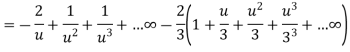
Hence
Which is valid in the region 1 < z + 1 < 3 |

Key takeaways-
2. Laurent’s series-
Where
|


A point at which a function f(z) is not analytic is known as a singular point or singularity of the function.
Isolated singular point- If z = a is a singularity of f (z) and if there is no other singularity within a small circle surrounding the point z = a, then z = a is said to be an isolated singularity of the function f (z); otherwise it is called non-isolated.
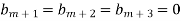
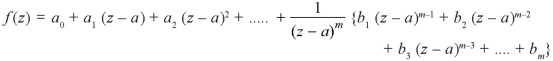
Pole of order m- Suppose a function f(z) have an isolated singular point z = a, f(z) can be expanded in a Laurent’s series around z = a, giving
In some cases it may happen that the coefficient
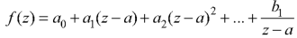
Then z = a is said to be a pole of order m of the function f(z). Note- The pole is said to be simple pole when m = 1. In this case-
Working steps to find singularity- Step-1: If Step-2: If Step-3: If |


Example: Find the singularity of the function-
|

Sol.
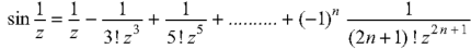
As we know that-
So that there is a number of singularity.
(1/z = ∞ at z = 0) |

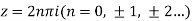
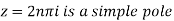
Example: Find the singularity of
|
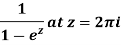
Sol.
Here we have-
We find the poles by putting the denominator equals to zero. That means-
|


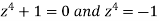
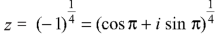
Example: Determine the poles of the function-
|

Sol.
Here we have-
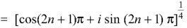
We find the poles by putting the denominator of the function equals to zero- We get-
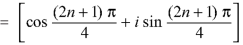
By De Moivre’s theorem-
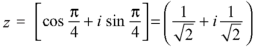
If n = 0, then pole-
If n = 1, then pole-
If n = 2, then pole-
If n = 3, then pole-
|

Cauchy’s residue theorem-
If f(z) is analytic in a closed curve C, except at a finite number of poles within C, then-
|

;DOProof:
Suppose  be the non-intersecting circles with centres at
  respectively.
Redii so small that they lie within the closed curve C. then f(z) is analytic in the multipUYle connected region lying between the curves C and
Now applying the Cauchy’s theorem-
|


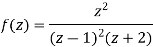
Example: Find the poles of the following functions and residue at each pole:
|
and hence evaluate-
|
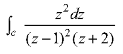
Sol.
The poles of the function are-
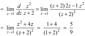
The pole at z = 1 is of second order and the pole at z = -2 is simple- Residue of f(z) (at z = 1)
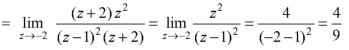
Residue of f(z) ( at z = -2)
|


Example: Evaluate-
|

Where C is the circle |z| = 4.
Sol.
Here we have,
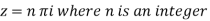
Poles are given by-
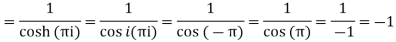
Out of these, the poles z = -πi , 0 and πi lie inside the circle |z| = 4. The given function 1/sinh z is of the form Its poles at z = a is Residue (at z = -πi)
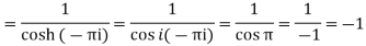
Residue (at z = 0)
Residue (at z = πi)
Hence the required integral is =
|


Key takeaways-
- The pole is said to be simple pole when m = 1.
- Cauchy’s residue theorem-
If f(z) is analytic in a closed curve C, except at a finite number of poles within C, then-
|
References
- E. Kreyszig, “Advanced Engineering Mathematics”, John Wiley & Sons, 2006.
- P. G. Hoel, S. C. Port And C. J. Stone, “Introduction To Probability Theory”, Universal Book Stall, 2003.
- S. Ross, “A First Course in Probability”, Pearson Education India, 2002.
- W. Feller, “An Introduction To Probability Theory and Its Applications”, Vol. 1, Wiley, 1968.
- N.P. Bali and M. Goyal, “A Text Book of Engineering Mathematics”, Laxmi Publications, 2010.
- B.S. Grewal, “Higher Engineering Mathematics”, Khanna Publishers, 2000.
- T. Veerarajan, “Engineering Mathematics”, Tata Mcgraw-Hill, New Delhi, 2010
- Higher engineering mathematics, HK Dass


