Unit 4
Series solution of Ordinary Differential Equations and Special Functions
We know that the solution of the differential equation-
Are
|

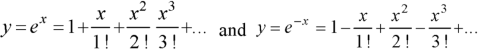
These are the power series solutions of the given differential equations.
Ordinary Point-
Let us consider the equation-
|
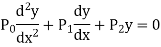
Here  are polynomial in x.
X = a is an ordinary point of the above equation if  does not vanish for x = a.
Note- If  vanishes for x = a, then x = a is a singular point.
Solution of the differential equation when x = 0 is an ordinary point, which means  does not vanish for x = 0.
1. Let 2. Find 3.
4. Substitute the expressions of y, 5. Calculate 6. Put the values of |


Example- Solve
|
Sol.
Here we have-
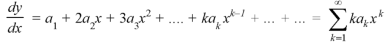
Let the solution of the given differential equation be-
Since x = 0 is the ordinary point of the given equation-
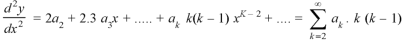
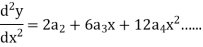
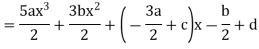
Put these values in the given differential equation-
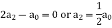
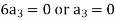
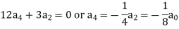
Equating the coefficients of various powers of x to zero, we get-
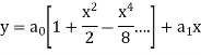
Therefore, the solution is-
|
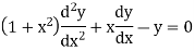


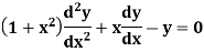
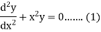
Example: Solve in series the equation-
|

Sol.
Here we have-
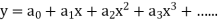
Let us suppose-
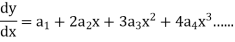
Since x = 0 is the ordinary point of (1)- Then-
And
Put these values in equation (1)- We get-
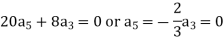
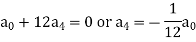
Equating to zero the coefficients of the various powers of x, we get-
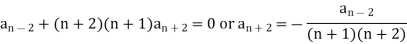
And so on…. In general, we can write-
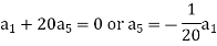
Now putting n = 5,
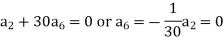
Put n = 6-
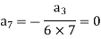
Put n = 7,
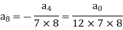
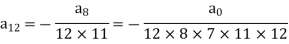
Put n = 8,
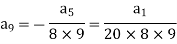
Put n = 9,
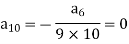
Put n = 10,
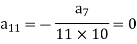
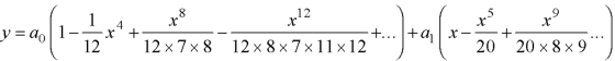
Put the above values in equation (1), we get-
|


Frobenius method-
This method is also called generalized power series method.
If x = 0 is a regular singularity of the equation.
|
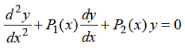
Then the series solution is-
|

Which is called Frobenius series.
On equating the coefficient of lowest power of x in the identity to zero, we get a quadratic equation in ‘m’.
We will get two values of m. The series solution of (1) will depend on the nature of the roots of the indicial equation-
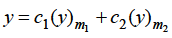
Case-1: when roots m1 and m2 are distinct and these are not differing by an integer- The complete solution in this case will be-
Case-2: when roots m1 and m2 are equal-
Case-3: when roots are distinct but differ by an integer-
Case-4: Roots are distinct and differing by an integer, making some coefficient indeterminate-
|
Example: Find solution in generalized series form about x = 0 of the differential equation
|
Sol.
Here we have
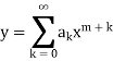
Since x = 0 is a regular singular point, we assume the solution in the form
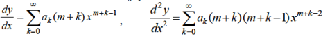
So that
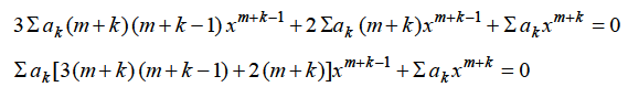
Substituting for y,
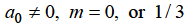
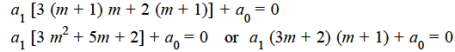
The coefficient of the lowest degree term = 0 in first summation only and equating it to zero. Then the indicial equation is
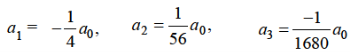
Since The coefficient of next lowest degree term k = 1 in first summation and k = 0 in the second summation and equating it to zero.
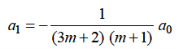
Equating to zero the coefficient of
Or
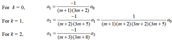
Which gives-
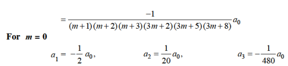
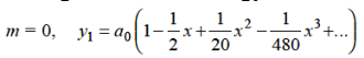
Hence for-
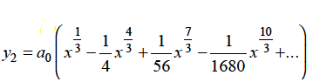
Form m = 1/3-
Hence for m = 1/3, the second solution will be-
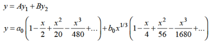
The complete solution will be-
|


Key takeaways
If x = 0 is a regular singularity of the equation.
Then the series solution is-
Which is called Frobenius series. |


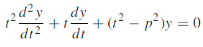
The Bessel equation is-
|
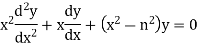
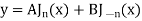
The solution of this equations will be-
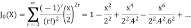
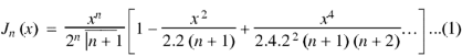
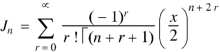
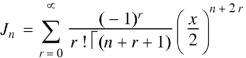
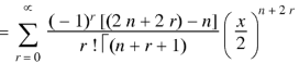
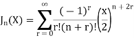
The Bessel function is denoted by  and defined as-
If we put n = 0 then Bessel function becomes-
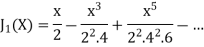
Now if n = 1, then-
|

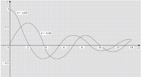
The graph of these two equations will be-
|
General solution of Bessel equation-
|

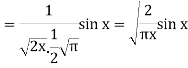
Example: Prove that-
|
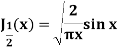
Sol.
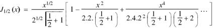
As we know that-
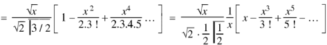
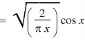
Now put n = 1/2 in equation (1), then we get-
Hence proved. |
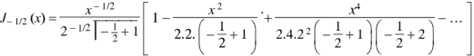
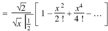
Example: Prove that-
|
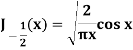
Sol.
Put n = -1/2 in equation (1) of the above question, we get-
|
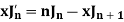
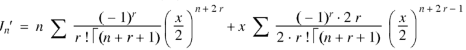
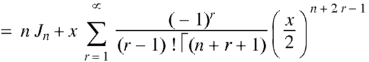
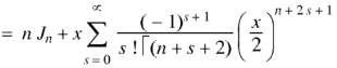
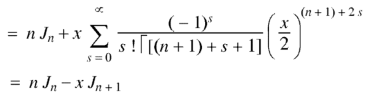
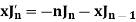
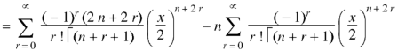
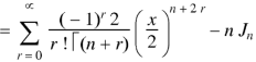
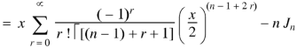
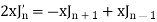
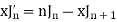
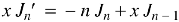
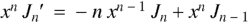
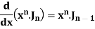
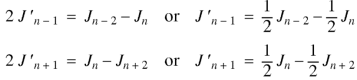
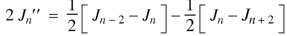
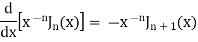
Recurrence formulae-
Formula-1:
|
Proof:
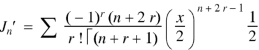
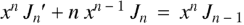
As we know that-
On differentiating with respect to x, we obtain-
Putting r – 1 = s
|
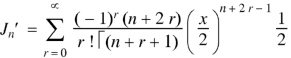
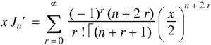
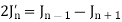
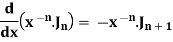
Formula-2:
|
Proof:
We have-
Differentiating w.r.t. x, we get-
|
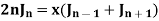
Formula-3:
|
Proof:
We know that from formula first and second-
Now adding these two, we get-
Or
|
Formula-4:
|

Proof:
We know that-
On subtracting, we get-
|
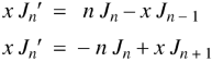

Formula-5:
|

Proof:
We know that-
Multiply this by
I.e.
Or
|


Formula-6:
|

Proof:
We know that-
Multiply by
Or
|

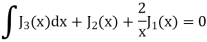
Example: Show that-
|

By using recurrence relation.
Sol.
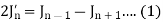
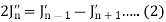
We know that- The recurrence formula-
On differentiating, we get-
Now replace n by n -1 and n by n+1 in (1), we have-
Put the values of
|


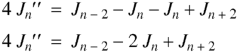
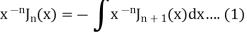
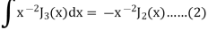
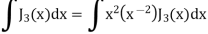
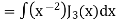
Example: Prove that-
|
Sol.
We know that- from recurrence formula
On integrating we get-
On taking n = 2 in (1), we get-
Again-
Put the value of
By equation (1), when n = 1
|


Key takeaways
2. General solution of Bessel equation-
|

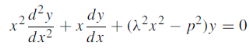
The differential equation
Where
Where-
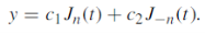
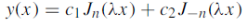
For p non-integral, the general solution of Equation (2) is
Thus the general solution of Equation (1) is
When p is non-integral. |


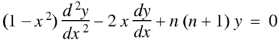
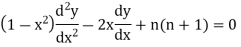
The Legendre’s equations is-
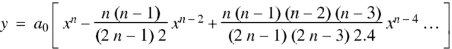
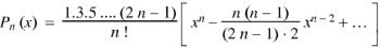
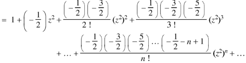
Now the solution of the given equation is the series of descending powers of x is-
Here If n is a positive integer and
The above solution is So that-
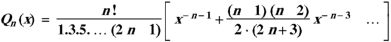
Here Note- Legendre’s equations of second kind is
The general solution of Legendre’s equation is-
Here A and B are arbitrary constants. |


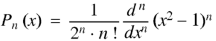
Rodrigue’s formula-
Rodrigue’s formula can be defined as-
|
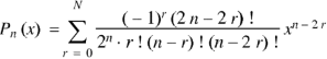
Legendre Polynomials-
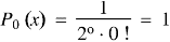
We know that by Rodrigue formula-
If n = 0, then it becomes-
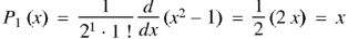
If n = 1,
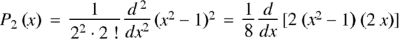
If n = 2,
Now putting n =3, 4, 5……..n we get-
…………………………………..
Where N = n/2 if n is even and N = 1/2 (n-1) if n is odd.
|

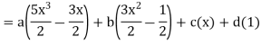
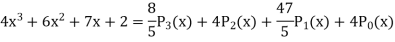
Example: Express
|
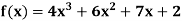
in terms of Legendre polynomials.
Sol.
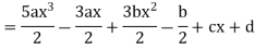
By equating the coefficients of like powers of x, we get-
Put these values in equation (1), we get-
|

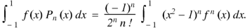
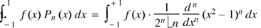
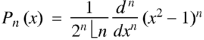
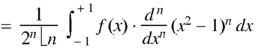
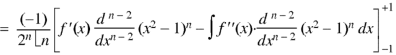
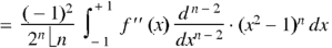
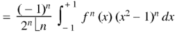
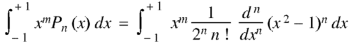
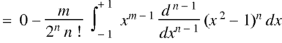
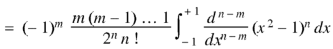
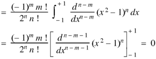
Example: Let  be the Legendre’s polynomial of degree n, then show that for every function f(x) for which the n’th derivative is continuous-
|
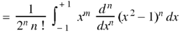
Sol.
We know that-
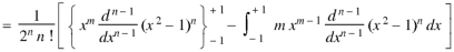
On integrating by parts, we get-
Now integrate (n – 2) times by parts, we get-
|
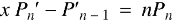
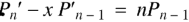
Recurrence formulae for  -
-
Formula-1:
Fromula-2:
Formula-3:
Formula-4:
Formula-5:
Formula-6:
|


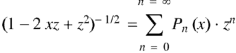
Generating function for 
Prove that  is the coefficient of
  in the expansion of
|
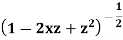
in ascending powers of z.
Proof:
Now coefficient of
Coefficient of
Coefficient of
And so on. Coefficient of
The coefficients of Therefore-
|


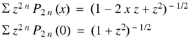
Example: Show that-
|
Sol.
We know that
Equating the coefficients of
|

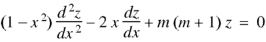
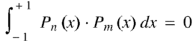
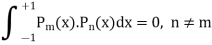
Orthogonality of Legendre polynomials-
|

Proof:
And
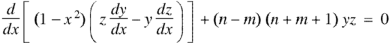
Now multiply (1) by z and (2) by y and subtracting, we have-
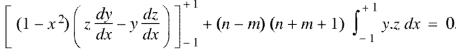
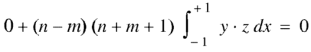
Now integrate from -1 to +1, we get-
|


Example: Prove that-
|

By using Rodrigue formula for Legendre function.
On integrating by parts, we get-
Now integrating m – 2 times, we get-
|

Key takeaways
2. The general solution of Legendre’s equation is-
Here A and B are arbitrary constants. 3. Rodrigue’s formula can be defined as-
4. Orthogonality of Legendre polynomials-
|

References
- E. Kreyszig, “Advanced Engineering Mathematics”, John Wiley & Sons, 2006.
- P. G. Hoel, S. C. Port And C. J. Stone, “Introduction To Probability Theory”, Universal Book Stall, 2003.
- S. Ross, “A First Course in Probability”, Pearson Education India, 2002.
- W. Feller, “An Introduction To Probability Theory and Its Applications”, Vol. 1, Wiley, 1968.
- N.P. Bali and M. Goyal, “A Text Book of Engineering Mathematics”, Laxmi Publications, 2010.
- B.S. Grewal, “Higher Engineering Mathematics”, Khanna Publishers, 2000.
- T. Veerarajan, “Engineering Mathematics”, Tata Mcgraw-Hill, New Delhi, 2010
- Higher engineering mathematics, HK Dass


