UNIT - 3
Time Response of feedback control systems
The Impulse signal, Ramp signal, unit step and parabolic signals are used as the standard test signals. All these signals are explained below.
Impulse Signal:-
This signal have zero amplitude everywhere expect at the origin. fig below shown the representation of Impulse signal.
|
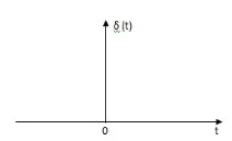
Fig 1 Impulse Signal
The mathematical representations
A (t) = 0 for t ≠0
 dt = A e
Where A represent energy or area of the Laplace Transform of Impulse signal is
L [A (t) ]= A
The transfer function of a linear time invariant System is the Laplace transform of the impulse response of the system. If a unit impulse signal is applied to system then Laplace transform of the output c(s) is the transfer function G(s)
As we know G(s) = c(s)/R(S)
r(t) =  (t)
(t)
R(s) = L [ (t)] = 1
:. G(S) = C(s)
(b) Step signal:-
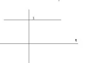
Step signal of size A is a signal that change from zero level to A in zero time and stays there forever.
|
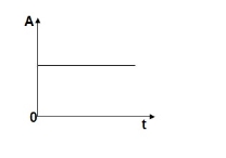
Fig 2 Unit Step Signal
r(t)= A t >=0
=0 t<0
L[r(t)]= R(s) = A/s
(c) Ramp Signal:-
|
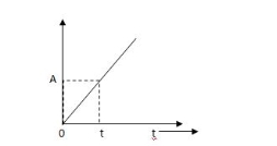
Fig 3 Ramp Signal
The vamp signal increase linearly with time from initial value of zero at t= 0 as shown in fig is below.
r(t) = At t>=0 =0 t<0 A is the slope of the line The Laplace transform of ramp signal is L[r(t)] = R(s) = A/s2
|
(d) Parabolic Signal:
The instantaneous value of a parabolic signal varies as square of the time from an initial value of zero t=0. The signal representation in fig 14 below.
|
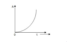
Fig 4 Parabolic Signal
r(t) At2 t>=0
=0 t<0
Then Laplace Transform is given as
R(s) = L[At2] = 2A/s3
CLTF c(s)/R(s) = 1/1+TS
CE: HTS = 0
S= -1/T
C(s) = R(s) [G(S)/1+G(s)]
C(s) = R(s)/1+TS
So, Calculating value of c(s), c(t) for different input
a) Unit Step: R(t) = u(t) R(s) = 1/s C(s) = 1/s(1+ST) 1/s(1+ST) = A/s + o/1+TS 1/s(1+ST) = A/S + 0/1+TS 1= A(1+ST) + BS AT +B =0 A = 1 B= -T C(s) = 1/s + (-T)/1+TS = 1+ (-T)/1-(-T)s = 1-I/n/1+ass+1/T =e-t/s C(t) = [ 1-e-t/T] | |
| |
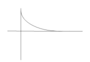
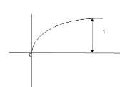
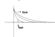
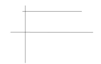
Fig 5 Output response for Unit Step input
Ramp:
R(t) = t R(s) = 1/s2 C(s) = R(s) [G(s)/1+G(s)] C(s) = 1/s2 1/(1+TS) + c 1/s2 (1+TS) = A/(s) + B/s2 + c(1+TS) 1 = A (s+s2. T) + B(1+TS) +cs2 TA +c = 0 A+TB =0 B =1 A = -T C = T2 C(s) = -T/s + 1/s2 +T2/1+ST =(-T) u(t) + t(u) + T e-t/T u(t) = [ -T + t +Te-t/T u(t) = [ -T+ t+Te-t/T] u(t) C(s) = t- T+ Te-t/T ess = = = ess = The less the value of T the less in the errors. |


|
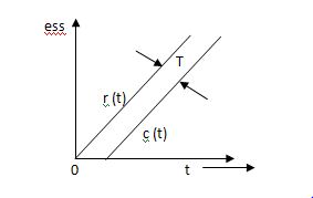
Fig 6 Output response for ramp input
Unit Step Ramp c(t) = 1-e-t/T r(t) = t ess = e-t/T (r/t)-(t) c(t) = t- T+te-t/T ess= e-t/T (r/t) (t) ess = T- Te-t/T for ess =0 ess = T
|


1) In both the vases (values of T) must be as small as possible (so, that e-t/T) must be as small as possible which gives us
|
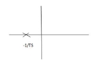
Fig 7 Location of poles
G(s) = 1/Ts
aTf = 1/1+TS
1st order system
Poles must be situated as far as possible from origin i.e. deeper and deeper into the left half of s-place. Thus, we get less errors.
Key takeaways
- From both the Cases input unit step, ramp Unit step
Specifications:
1) Rise Time (tp):- The time taken by the output to reach the already status value for the first time is known as Rise time.
C(t) = 1-e- wnt/
wnt/ 1-
1- 2 sin (wdt+ø)
Sin (wd +ø) = 0
Wdt +ø = n
tr =n -ø/wd
-ø/wd
for first time so ,n=1.
2) Peak Time (tp)
The peak value attained by the output is called peak time. The time required by the output to reach this value is lp.
d(cct) /dt = 0 (maxima)
d(t)/dt = peak value
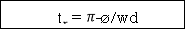
tp = n /wd for n=1
tp =  wd
wd
3) Peak Overshoot Value:
Maximum deviation of output from steady state value is called peak overshoot value (Mp).
(ltp) = 1 = Mp ( ( Mp = e-∏ξ / √1 –ξ2
|

Condition 3 ξ = 1
C( S ) = R( S ) Wn2 / S2 + 2ξWnS + Wn2 C( S ) = Wn2 / S(S2 + 2WnS + Wn2) [ R(S) = 1/S ] C( S ) = Wn2 / S( S2 + Wn2 ) C( t ) = 1 – e-Wnt + tWne-Wnt |
The response is critically damped.
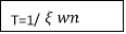
(4). Settling Time (ts) :
ts = 3 / ξWn ( 5% )
ts = 4 / ξWn ( 2% )
Key takeaways
- Rise Time tr =
 -ø/wd
-ø/wd - Peak Time tp = n
 /wd for n=1
 - tp =
 wd
wd - Peak Overshoot Value
- Mp% = e-∏ξ / √1 –ξ2
- Settling Time
ts = 3 / ξWn ( 5% )
ts = 4 / ξWn ( 2% )
OLTF G(s) = k/s(1+TS)
CLTFC(s)/R(s) = k/k+s(1+Ts)
= k/s2+ s/T +k/T
Comparing above equation with standard 2nd order eqn CEs2+2 S= -2 =2 S= S= - S= - S= -
Standard eqn:- T(s) = wn2/s2+2 Our eqn T(s) = K/T/s2+1/T s+ K/T Wn2 = k/T 2 2
Graphically showing the position of loops s1,s2 for offered of As the characteristic Equn (location of poles) is dependent only on (wn constant for a given system) S1 = - S2= -
|


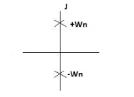
CASE 1: ( =0)
=0)
S1=jwn,S2, = -jwn
|
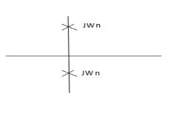
Fig 8 Location of poles for  =0
=0
Undamped
CASE 2:(0< <1)
<1)
S1= -wn + jwn  0.75
0.75
=-wn/2 +jwn(0.26)
S2 = -wn/2 – jwn (0.86)
|
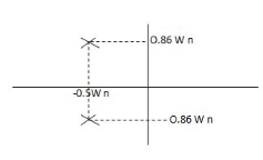
Fig 9 Location of poles for  <1
<1
CASE:3 ( =1)
=1)
S1= S2 = - wn = -wn
|
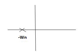
Fig 10 Location of poles for  =1
=1
CASE4:- ( =-2)
=-2)
S1 = -2wn +jwn  -3
-3
=-2wn – jwn (1.73)
S1 = -3.73wn
S2 = -2wn –jwn  -3
-3
= -2wn + jwn (1.73)
= -0.27  wn
wn
|
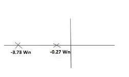
Fig 11 Location of poles for  >1
>1
Overdamped
CLTF = e(s)/ R(s) = wn2/s2+2 wns+wn2
Now calculating c(s) , c(t) for different values of input
1) Impulse I/p R(t) = R(s) = 1 C(s) = R(s) wn2/s2+2 C(s) = wn2/s2 +2 Under this i/p (R(t) =
|


CONDITION 1: ( =0)
=0)
C(s) =wn2/s2 +wn2
os2 +wn2 =0
S=+-jwn
C(t) = wn sinwnt
|
Sinwnt
|
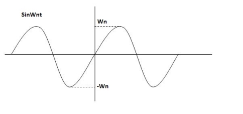
Fig 12 Undamped oscillations
As there in no damping i.e. oscillations at t= 0 are some at t CONDITION 2: 0<<1 c(s) = R(s) wn2/s22 R(s) =1 C(s) = wn2/s2+2 CE S2+2 S2, S1 = - |


|
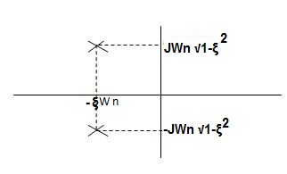
C(t) = e- wnt sin( wn
  )t
)t
C(t)=e- wnt sin (wdt)
|
|
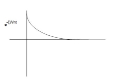
Fig 13 Underdamped oscillations
The oscillations are present but at t- infinity the Oscillations are 0 so, it is UNDERDAMPED
CONDITION 3 : =1
=1
C(s) = R(s) wn2/s2+2 wns+wn2
C(s)=wn2/S2 +2wns+wn2
=wn2/(s +wn)2
CE S= -Wn
Diagram
C(t)= w2n /(
 )2
)2
C(t)=
|
|
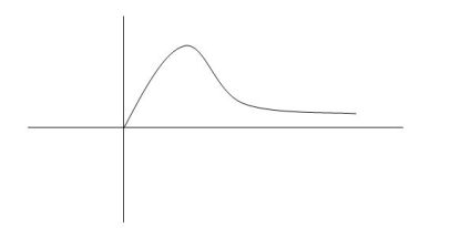
Fig 14 Critically damped oscillations
No damping obtained at  so is called CRITICALLY DAMPED.
CONDITIONS 4 :- >1
>1
C(s) = wn2/s22 wnS+Wn2
S1,s2 =  WN+-jwn
|
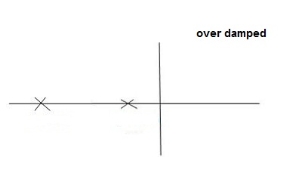
Fig 15 location of poles for over damped oscillations
b) UNIT Step Input:
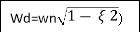
R(s) = 1/s C(s)/R(s) = wn2/s2+2 C(s) = R(s) wn2 /s2 +2 C(s) = R(s) wn2/s2+2 C(s) = R(s) wn2/s2+2 C(s) = wn2s(s2+2 C(t) = 1- e Wd = wn Ø= Where Wd = Damping frequency of oscillations Wn = natural frequency of oscillations
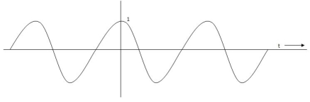
T= Time constant Condition 1 C(s) = wn2 /s(s2+wn2) C(t) = 1- e° sin wdt +ø C(t)= 1- sin( wn +90) C(t) = 1+cos wnt Constant
|


|
|
C(t) = 1+constant
|
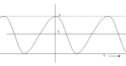
Fig 16 C(t) = 1+cos wnt
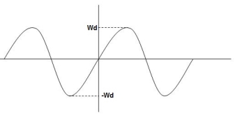
Condition 2:- 0< C(s) = C(s) =1/s – s+ =1/s – s+ Wd = wn Taking Laplace inverse of above equation L --1 s+ L-1 s+ C(t) = 1-e- = 1-e C(t) = 1-e Ø = |


|
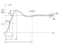
Fig 17 Transient Response of second order system
Key takeaways
- All practical systems are 2 order to, if R(e) =
 (t) R(s) = 1:. CLTF = 2nd order standard eqn and hence already the system is possible.
Q.1. The open loop transfer function of a system with unity feedback gain G( S ) = 20 / S2 + 5S + 4. Determine the ξ, Mp, tr, tp.
Soln:
Finding closed loop transfer function,
C( S ) / R( S ) = G( S ) / 1 + G( S ) + H( S )
As it is unity feedback so, H(S) = 1
C(S)/R(S) = G(S)/1 + G(S)
= 20/S2 + 5S + 4/1 + 20/S2 + 5S + 4
C(S)/R(S) = 20/S2 + 5S + 24
Standard equation for 2nd order system,
S2 + 2ξWnS + Wn2 = 0
We have,
S2 + 5S + 24 = 0
Wn2 = 24
Wn = 4.89 rad/sec
2ξWn = 5
(a). ξ = 5/2 x 4.89 = 0.511
(b). Mp% = e-∏ξ / √1 –ξ2 x 100
= e-∏ x 0.511 / √1 – (0.511)2 x 100
Mp% = 15.4%
(c). tr = ∏ - φ / Wd
φ = tan-1√1 – ξ2 / ξ
φ= tan-1√1 – (0.511)2 / (0.511)
φ = 1.03 rad.
tr = ∏ - 1.03/Wd
Wd = Wn√1 – ξ2
= 4.89 √1 – (0.511)2
Wd = 4.20 rad/sec
tr = ∏ - 1.03/4.20
tr = 502.34 msec
(d). tp = ∏/4.20 = 747.9 msec
Q.2. A second order system has Wn = 5 rad/sec and is ξ = 0.7 subjected to unit step input. Find (i) closed loop transfer function. (ii) Peak time (iii) Rise time (iv) Setteling time (v) Peak overshoot.
Soln:
The closed loop transfer function is
C(S)/R(S) = Wn2 / S2 + 2ξWnS + Wn2
= (5)2 / S2 + 2 x 0.7 x S + (5)2
C(S)/R(S) = 25 / S2 + 7s + 25
(ii). tp = ∏ / Wd
Wd = Wn√1 - ξ2
= 5√1 – (0.7)2
= 3.571 sec
(iii). tr = ∏ - φ/Wd
φ= tan-1√1 – ξ2 / ξ = 0.795 rad
tr = ∏ - 0.795 / 3.571
tr = 0.657 sec
(iv). For 2% settling time
ts = 4 / ξWn = 4 / 0.7 x 5
ts = 1.143 sec
(v). Mp = e-∏ξ / √1 –ξ2 x 100
Mp = 4.59%
Q.3. The open loop transfer function of a unity feedback control system is given by
G(S) = K/S(1 + ST)
Calculate the value by which k should be multiplied so that damping ratio is increased from 0.2 to 0.4?
Soln: C(S)/R(S) = G(S) / 1 + G(S)H(S) H(S) = 1 C(S)/R(S) = K/S(1 + ST) / 1 + K/S(1 + ST) C(S)/R(S) = K/S(1 + ST) + K C(S)/R(S) = K/T / S2 + S/T + K/T For second order system, S2 + 2ξWnS + Wn2 2ξWn = 1/T ξ = 1/2WnT Wn2 = K/T Wn =√K/T ξ = 1 / 2√K/T T ξ = 1 / 2 √KT forξ1 = 0.2, for ξ2 = 0.4 ξ1 = 1 / 2 √K1T ξ2 = 1 / 2 √K2T ξ1/ ξ2 = √K2/K1 K2/K1 = (0.2/0.4)2 K2/K1 = 1 / 4 K1 = 4K2 |
Q.4. Consider the transfer function C(S)/R(S) = Wn2 / S2 + 2ξWnS + Wn2
Find ξ, Wn so that the system responds to a step input with 5% overshoot and settling time of 4 sec?
Soln:
Mp = 5% = 0.05
Mp = e-∏ξ / √1 –ξ2
0.05 = e-∏ξ / √1 –ξ2
Cn 0.05 = - ∏ξ / √1 –ξ2
-2.99 = - ∏ξ / √1 –ξ2
8.97(1 – ξ2) = ξ2∏2
0.91 – 0.91 ξ2 = ξ2
0.91 = 1.91 ξ2
ξ2 = 0.69
(ii). ts = 4/ ξWn
4 = 4/ ξWn
Wn = 1/ ξ = 1/ 0.69
Wn = 1.45 rad/sec
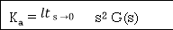
So, for difficult input, ess will be different Input still be 1) R(s) = unit step
2) R (s) = Ramp 3) R(s) = parabolic 1) R(s)= Unit step R(t) = u(t) R(s) = 1/s ess = = ess=
(Position error coefficient)
1) R(s) = Ramp R(t) = t R(s) = 1/s2 ess= = = = ess =
(3)Parabolic R(t) = t2 R(s) =1/s3 ess = = =
Acceleration error coefficient
Now finding errors in type 0,1,2 system 1) Type 0:- G(s) = 1/(s+a) (s+b) 2) Kp : Kp = = Kp= 1/ab ess=1/1+np = 1/1+(1/ab) o/p not locking the input (b) kv:- Kv =
= = kv = 0 ess = 1/kv = o/p not locating the input (3)ka:- ka = = Ka =0 ess = 1/ka = o/p not locking the input (2)Type –I :- G(s) = 1/s(s+a) (s+b) Kp = = Kp = 1/0 = ess = 1/1+kp = 0 o/p is tracking the input (b)kv:- Kv = = =1/ab Kv = 1/ab ess =1/ka = ab o/p is not tracking the input 3)ka : Ka= = = Ka= 0 ess = 1/ka = O/p is not tracking the input . 3) Type 2 :- G(s) = 1+/(s2(s+a) (s+b) a) Kp:- Kp = = Kp = ess = 1/1+kp = 0 o/p tracking the i/p b) kv:- Kv = = kv = ess =1/ o/p tracking the o/p (b) ka:- Ka= = ka = 1/ab ess = 1/(yab) ≠0 o/p not locking the i/p Key takeaway:
|


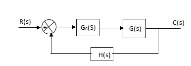
Effects of controller are viewed on time response and stability.
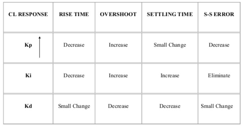
Fig 18 Controller with unity feedback system Gc(S) = TF of the controller G(S) = OLTF without controller G’(S) = Gc(S).G(S) = OLTF with controller 1. Proportional (P) Controller – Proportional means scalar Multiplier. Gc(S) = Kp Stability can be controlled Q. G(S) = 1/S(S + 8) CLTF = 1/S2 + 8S + 1 w2n = 1 wn = 1 2ξWn = 8 ξ = 4 ξ>/1 so, overdamped. Now introducing Gc(S) = K G’(S) = Kp/S(S + 8) CLTF = Kp/S2 + 8S + Kp wn = √Kp 2 ξwn = 8 ξ = 4/√Kp If, Kp = 16; ξ = 1; critically damped Kp> 16; ξ< 1; undamped Kp< 16; ξ> 1; overdamped
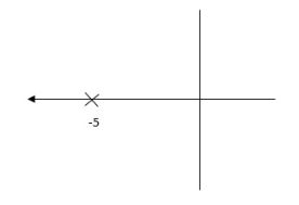
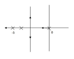
2. Integral (I) controller – The transfer function of this controller is Gc(S) = Ki/S Integral controller is used to improve the steady state response or reduce the steady state error.
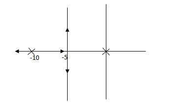
Fig 19 Integral Controller G’(S) = Gc(S).G(S) G(S) = 1/S + 5, Gc(S) = Ki/S G’(S) = Ki/S(S + 5). After applying the Gc(S) the type of system is increasing and hence, the steady state error is decreasing (Refer Time Response). Disadvantage - By using integral controller, the stability of closed loop system decreases. G(S) = 1/S + 5
Fig 20 Pole Locations For given system G’(S) = Ki/S(S + 5)
Fig 21 Pole Location after Integral controller
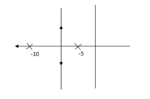
Fig(20), is more stable than (21) as more the away the pole from origin (imaginary axis) more is the stability. Q. G(S) = 1/(S + 5)(S + 10) G’(S) = Kp/S(S + 5)(S + 10) G(S) = 1/(S + 5)(S + 10)
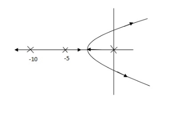
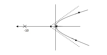
Fig 22 Root Locus Without controller G’(S) = Ki/S(S + 5)(S + 10)
Fig 23 Root Locus Without controller So, Fig 23 is less stable at root locus lies on the R.H.S,
3. Derivative (D) Controller - They are used to improve the stability.
Fig 24 Derivative controller system G’(S) = KdS/S2(S + 10)
Fig 25 Root Locus for system without controller
Fig 26 Root locus with controller Fig 26 is stable i.e. more stable than the Fig 25.
Disadvantage – It increases the steady state i.e. o/p will not track the input at steady state.
4. Proportional Plus Integral [PI] controller -
Fig 27 PI controller Gc(S) = KpS + Ki/S The steady state error will decrease and the stability will depend on Kp i.e. if Kp is increased/decreased than according to it stability will change (Kpα stability). Used to reduce ess without much affecting the stability. 5. Proportional Plus Derivative (PD) Controller -
Fig 28 PD controller Used to improve the stability without affecting much the steady state error.
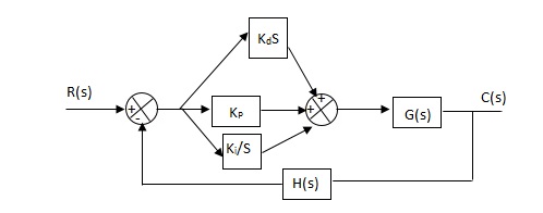
6. PID controller - Gc(S) = Kp + Ki/S + KdS
Fig 29 PID Controller It improves the stability. It decreases the steady state error and both are proportional to Kp.
Key takeaway
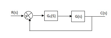
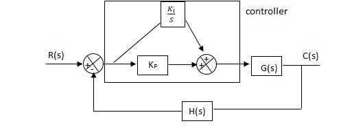
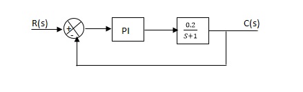
Que) The block diagram of a system using PI controllers is shown in the figure 30 Calculate: (a). The steady state without and with controller for unit step input? (b). Determine TF of newly constructed sys. With controller so, that a CL Poles is located at -5?
Fig 30 Block diagram with PI controller (a). Without : C(S)/R(S) = 0.2/(S + 1) C(S) = R(S) 0.2/(S + 1) + 0.2 For unit step ess = 1/1 + Kp Kp = lt G(S) S 0 = lt 0.2/(S + 1) S 0 Kp = 0.2 ess = 1/1.2 = 5/6 = 0.8 (b). With controller :
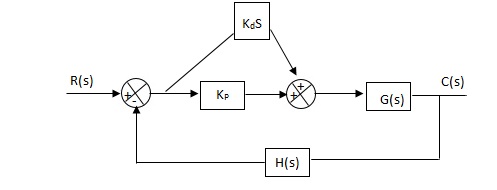
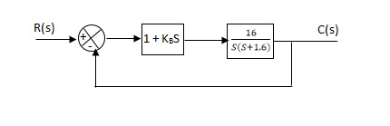
Q.The block diagram of a system using Pd controller is shown, the PD is used to increase ξ to 0.8. Determine the T.F of controller?
Fig 31 Block diagram with PD controller (1). Kp = 1 Without controller:- C(S)/R(S) = 16/S2 + 1.6S + 16 wn = 4 2 ξwn = 16 ξ = 1.6/2 x 4 = 0.2 (b). With derivative :- ξS = 0.2 to 0.8 undamped to critically damped, G’(S) = (1 + KdS)(16)/(S2 + 1.6S) CE: S2 + 1.6S + 16(1 + KdS) = 0 S2 + (1.6 + Kd)S + 16 = 0 2 ξwn = 1.6 + Kd1.6 wn = 4 ξS = 0.8 2 x 4 x 0.8 = 1.6 + Kd1.6 6.4 – 1.6 = Kd1.6 4.8/16 = Kd Kd = 0.3 TF = (1 + 0.3S)16/S(S + 16) |

1. “Modern Control Engineering “, K. Ogata, Pearson Education Asia/
PHI, 4th Edition, 2002.
2. “Automatic Control Systems”, Benjamin C. Kuo, John Wiley India
Pvt. Ltd., 8th Edition, 2008.
3. “Feedback and Control System”, Joseph J Distefano III et al.,
Schaum’s Outlines, TMH, 2nd Edition 2007.
4. J. Nagarath and M.Gopal, “Control Systems Engineering”, New Age
International (P) Limited, Publishers, Fourth edition – 2005


