4.1 Concepts of stability | unit 4 stability analysis

Back to Study material

UNIT - 4

Stability analysis

4.1 Concepts of stability

A stable system always gives bounded output for bounded input and the system is known as BIBO stable

A linear time invariant (LTI) system is stable if,

The system is BIBO stable

In absence of the input the output tends towards zero

For system

1) R(S)

Fig 1 Control system with G(s) = 1/s2

For R(s) = 1

C(S) =

R (t) = (t) C (t) = t

R (t) (t)

T Bounded Unbounded

Fig 2 Input R(t) Fig 3 Input and output for

So, system unstable.

Eg.2 R(s)

[R(s) = 1]

C(t) = e-10t C(t)

t= 0

e-10t

e-10t C(t)

Fig 4 BIBO stable figure

4.2 Necessary conditions for Stability

Effect of location of Poles on stability

A) Real and negative G(s)=

C(t)

-a

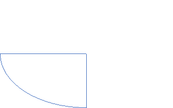
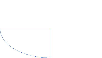
Fig 5 Output for G(s)=

Stable

B) Poles on right half of S- plane

G(s) =

Iw C(t)

0 t

Unstable: Unbounded Output

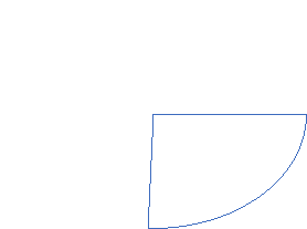
Fig 6 Input and Output for G(s) =

(C)Poles at origin

G(s)=

iw C(t)

Marginally stable

Fig 7 Input and output for G(s)=

4) Complex poles on left half of S-plane

S1,S2= -α ± iw

C(t) = k e- αt Cos wt

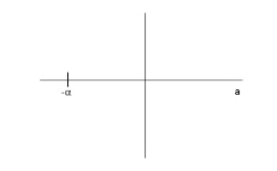
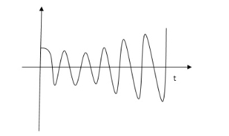
Fig 8 Pole location and output for C(t) = k e- αt Cos wt

At t - ∞ C(t) – 0 so, system stable

5) Complex poles on right half of S-plane

S1,S2 = α ± iw.

C(t) = k eαt COS wt.

C(t) increases exponentially with t ∞

So, unstable.

6) Poles on iw axis:

S1,S2 = ± iw.

C(t) = k COS wt.

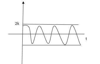
Fig 9 Output response of C(t) = k COS wt.

The system is marginally stable than sustained oscillations.

Key takeaways

Consider a system with characteristic equation

aoSm + a1 Sm-1 ……………..am=0.

2. All the coefficients of above equation should have same sign.

3. There should be no missing term.

The above two condition are necessary but not sufficient condition for stability

4.3 Routh- stability criterion, Relative stability analysis; More on the Routh stability criterion.

It states that the system is stable if and only if all the elements is the first column have the same algebraic sign. If all elements are not of the same sign then the number of sign changes of elements in first column equals the number of roots of the characteristic equation in the right half of S-plane.

Consider the following characteristic equation:

Continue the same procedure to find new rows.

a0 Sn + a1 Sn-1 ………….an = 0 where a0,a1,,,,,,,,,,,,,,,,,,,,an have same sign and are non-zero.

Step1 Arrange coefficients in rows

Row1 ao a2 a4

Row2 a1 a3 a5

Step2 Find third row from above two rows

Row1 a0 a2 a4

Row2 a1 a3 a5

Row3 a1 a3 a5

a1 = =

a3 = =

Q1) for the given polynomials below determine the stability of the system

S4+2S3+3S2+4S+5=0

1) Arranging Coefficient in Rows

S4	1	3	5
S3	2	4	0
S2	1	5	0
S1	-6	0	0
S0	5	0	0

For row S2 first term

S2 = = 1

For row S2 Second term

S2 = = 5

For row S1:

S1 = = -6

For row S0

S0 = = 5

As there are two sign change in the first column, So there are two roots or right half of S-plane making system unstable.

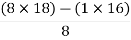
Q2. Using Routh criterion determine the stability of the system with characteristic equation S4+8S3+18S2+16S+S = 0

Sol :-

Arrange in rows.

S4	1	18	5
S3	8	16	0
S2	16	5
S1	13.5
S0	5

For row S2 first element

S1 = = 16

Second terms = = 5

For S1

First element = = 13.5

For S0

First element = As there is no sign change for first column so all roots are is left half of S-plane and hence system is stable.

Special Cases of Routh Hurwitz Criterions

When first element of any row is zero.

In this case the zero is replaced by a very small positive number

E and rest of the array is evaluated.

Eg.(1) Consider the following equation

S3+S+2 = 0

S3	1	1
S2	0	2
S1

Replacing 0 by E

S3	1	1
S2	E	2
S1		0
S0	2

Now when E 0, values in column 1 becomes

S3	1	1
S2	E	2
S1		0
S0	2

Two sign changes hence two roots on right side of S-plans

II) When any one row is having all its terms zero.

When array one row of Routh Hurwitz table is zero, it shown that the X is attests one pair of roots which lies radially opposite to each other in this case the array can be completed by auxiliary polynomial. It is the polynomial row first above row zero.

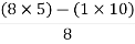
Consider following example

S3 + 5S2 + 6S + 30

S3	1	6
S2	5	30
S1	0	0
S0

For forming auxiliary equation, selecting row first above row hang all terms zero.

A(s) = 5S2 e 30

= 10s e0.

Again forming Routh array

S3	1	6
S2	5	30
S1	10
S0	30

No sign change in column one the roots of Auxiliary equation A(s)=5s2+ 30-0

5s2+30 = 0

S2 α 6= 0

S = ± j

Both lie on imaginary axis so system is marginally stable.

Q3. Determine the stability of the system represent by following characteristic equations using Routh criterion

1) S4 + 3s3 + 8s2 + 4s +3 = 0

2) S4 + 9s3 + 4S2 – 36s -32 = 0

1) S4+3s3+8s2+4s+3=0

S4	1	8	3
S3	3	4	0
S2	6.66	3
S1	2.650	0
S0	3

No sign change in first column to no rows on right half of S-plane system stable.

S4+9S3+4S2-36S-32 = 0

S4	1	4	-32
S3	9	-36	0
S2	8	-32
S1	0	0
S0

Special case II of Routh Hurwitz criterion forming auxiliary equation

A1 (s) = 8S2 – 32 = 0

= 16S – 0 =0

S4	1	4	-32
S3	9	-36	0
S2	8	-32
S1	16	0
S0	-32

One sign change so, one root lies on right half S-plane hence system is unstable.

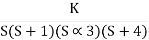
Q4. For using feedback open loop transfer function

G(s) =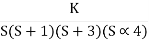

find range of k for stability

Soln:- Findlay characteristics equation .

CE = 1+G (s) H(s) = 0

H(s) =1 using feedback

CE = 1+ G(s)

1+ = 0

S(S+1)(S+3)(S+4)+k = 0

(S2+5)(S2+7Sα12)αK = 0

S4α7S3α1252+S3α7S2α125αK = 0

S4+8S3α19S2+125+k = 0

By Routh Hurwitz Criterion

S4	1	19	K
S3	8	12	0
S2	17.5	K
S1		0
S0	k

For system to be stable the range of K is 0< K < .

S4	1	12	K
S3	4	36
S2	3	K
S1
S0	K

Q5. The characteristic equation for certain feedback control system is given. Find range of K for system to be stable.

Soln

S4+4S3α12S2+36SαK = 0

For stability K>0

> 0

K < 27

Range of K will be 0 < K < 27

Relative Stability Criterion:

Routh stability criterion deals about absolute stability of any closed loop system. For relative stability we need to shift the S-plane and the apply the Routh criterion.

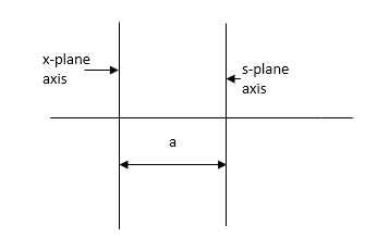
Fig 10 Location of Pole for relative stability

The above fig 10 shows the characteristic equation is modified by shifting the origin of S-plane to S1= -.

S = Z-S1

After substituting new valve of S =(Z-S1) applying Routh stability criterion, the number of sign changes in first column is the number of roots on right half of S-plane

Q6. Check if all roots of equation

S3+6S2+25S+38 = 0, have real poll more negative than -1.

Soln:-

S3	1	25
S2	6	38
S1	18.67
S0	38

No sign change in first column, hence all roots are in left half of S-plane.

Replacing S = Z-1. In above equation

(Z-1)3+6(Z-1)2+25(Z-1)+38 = 0

Z3+ Z23+16Z+18=0

Z3	1	16
Z2	3	18
Z1	10
Z0	18

No sign change in first column roots lie on left half of Z-plane hence all roots of original equation in S-domain lie to left half 0f S = -1

Key takeaway

Special Cases of Routh Hurwitz Criterions

When first element of any row is zero.

In this case the zero is replaced by a very small positive number E and rest of the array is evaluated.

2. When any one row is having all its terms zero.

3. When array one row of Routh Hurwitz table is zero, it shown that the X is attests one pair of roots which lies radially opposite to each other in this case the array can be completed by auxiliary polynomial. It is the polynomial row first above row zero.

References:

1. “Modern Control Engineering “, K. Ogata, Pearson Education Asia/

PHI, 4th Edition, 2002.

2. “Automatic Control Systems”, Benjamin C. Kuo, John Wiley India

Pvt. Ltd., 8th Edition, 2008.

3. “Feedback and Control System”, Joseph J Distefano III et al.,

Schaum’s Outlines, TMH, 2nd Edition 2007.

4. J. Nagarath and M.Gopal, “Control Systems Engineering”, New Age

International (P) Limited, Publishers, Fourth edition – 2005