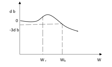
The transfer function of second order system is shown as C(S)/R(S) = W2n / S2 + 2ξWnS + W2n - - (1) ξ = Ramping factor Wn = Undamped natural frequency for frequency response let S = jw C(jw) / R(jw) = W2n / (jw)2 + 2 ξWn(jw) + W2n Let U = W/Wn above equation becomes T(jw) = W2n / 1 – U2 + j2 ξU so, | T(jw) | = M = 1/√(1 – u2)2 + (2ξU)2 - - (2) T(jw) = φ = -tan-1[ 2ξu/(1-u2)] - - (3) For sinusoidal input the output response for the system is given by C(t) = 1/√(1-u2)2 + (2ξu)2Sin[wt - tan-1 2ξu/1-u2] - - (4) The frequency where M has the peak value is known as Resonant frequency Wn. This frequency is given as (from eqn (2)). dM/du|u=ur = Wr = Wn√(1-2ξ2) - - (5) from equation(2) the maximum value of magnitude is known as Resonant peak. Mr = 1/2ξ√1-ξ2 - - (6) The phase angle at resonant frequency is given as Φr = - tan-1 [√1-2ξ2/ ξ] - - (7) As we already know for step response of second order system the value of damped frequency and peak overshoot are given as Wd = Wn√1-ξ2 - - (8) Mp = e- πξ2|√1-ξ2 - - (9)
|
The comparison of Mr and Mp is shown in figure(1). The two performance indices are correlated as both are functions of the damping factor ξ only. When subjected to step input the system with given value of Mr of its frequency response will exhibit a corresponding value of Mp.
|
|
|
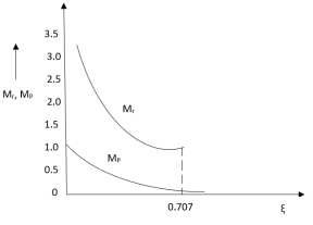
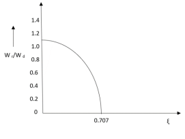
Fig 1 Frequency Domain Specification
Similarly the correlation of Wr and Wd is shown in fig(1) for the given input step response [ from eqn(5) & eqn(8) ]
Wr/Wd = √(1- 2ξ2)/(1-ξ2)
Mp = Peak overshoot of step response
Mr = Resonant Peak of frequency response
Wr = Resonant frequency of Frequency response
Wd = Damping frequency of oscillation of step response.
From fig(1) it is clear that for ξ> 1/2, value of Mr does not exists.
Key takeaway
- Mr and Mp are correlated as both are functions of the damping factor ξ only
- When subjected to step input the system with given value of Mr of its frequency response will exhibit a corresponding value of Mp.
In polar plot any point gives the magnitude phase of the transfer function in bode we split magnitude and  plot.
plot.
Advantages
Q. G(S) = 1. substitute S = j G(j M =
Magnitude varies with ‘w’ but phase is constant. MdB = +20 log10
|


Decade frequency:
W present = 10 Then
0.01 40 0.1 20 1 0 (shows pole at origin) 0 -20 10 -40 100 -60 Slope = (20db/decade) |


|
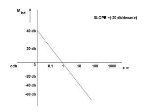
Fig 2 MAGNITUDE PLOT
|
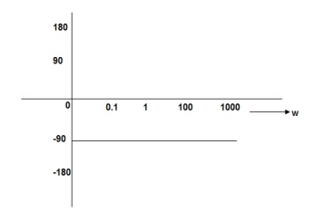
Fig 3 PHASE PLOT
Q.G(S) = 
G(j ) =
) = 
M =  ;
;  = -1800 (-20tan-1
 )
)
MdB = +20 log  -2
-2
MdB = -40 log10
 MdB
MdB
0.01 80
0.1 40
1 0 (pole at origin)
10 -40
100 -80
Slope = 40dbdecade
Q. G(S) = S
M= W
 = 900
= 900
MdB = 20 log10
 MdB
MdB
0.01 -40
0.1 -20
1 0
10 20
100 90
1000 60
|
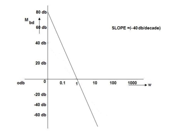
Fig 4 Bode Plot G(S) = S
Q. G(S) = S2
M=  2 MdB = 20 log10
 2
2
 = 1800 = 40 log10
W MdB
0.01 -80
0.1 -40
1 0
10 40
100 80
|
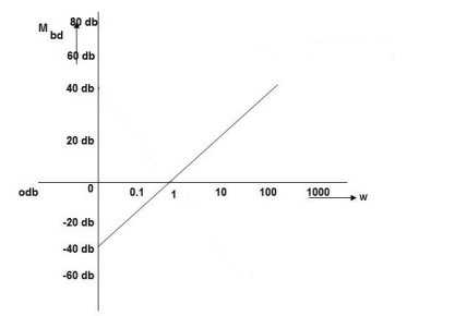
Fig 5 Magnitude Plot G(S) = S2
Q. G(S) = G(j M = MdB = 20 log10 K-20 log10
K=1 K=10
=-20 log10 0.01 40 60 0.1 20 40 1 0 20 10 -20 0 100 -40 -20 |


|
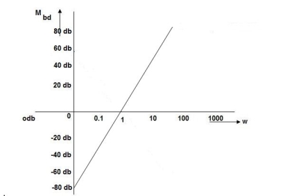
Fig 6 Bode Plot G(S) = 
|
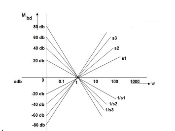
Fig 7 All bode plots in one plot
|
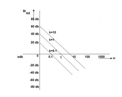
Fig 8 Variation in K shifts magnitude plot by +20db
As we vary K  then plot shift by 20 log10K i.e. adding a d.c. to a.c. quantity
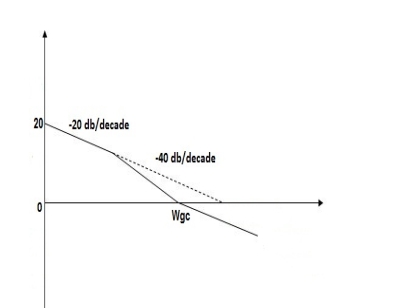
Approximation of Bode Plot:
IF poles and zeros are not located at origin G(S) = TF = M = MdB = -20 log10 (
Approximation: MdB = -20 log10 MdB = -20 log10 Approximation: MdB= 0dB, At a point both meet so equal i.e a time will come hence both approx become equal -20 log10
At this frequency both the cases are equal MdB = -20 log10 Now for MdB = -20 log10 = -20 log10 = -10 log102 MdB = 10 |


|
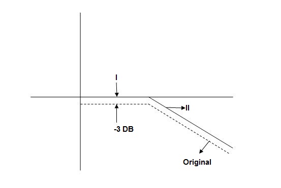
Fig 9 Approximation in bode plot
When we increase the value of  in app 2 and decrease the
  of app 1 so a RT comes when both cases are equal and hence for that value of
  where both app are equal gives max. error we found above and is equal to 3dB.
At corner frequency we have max error of -3dB
|


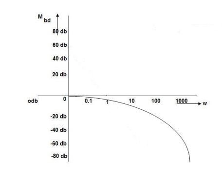
Fig 10 Magnitude Plot with approximation
Without approximation For second order system TF = TF = = = = M= MdB= Case 1 MdB= 20 log10 Case 2 MdB = -20 log10 = -20 log10 = -20 log10
MdB = -20 log10 = -40 log10 Case 3 . when case 1 is equal to case 2 -40 log10
The natural frequency is our corner frequency |


|
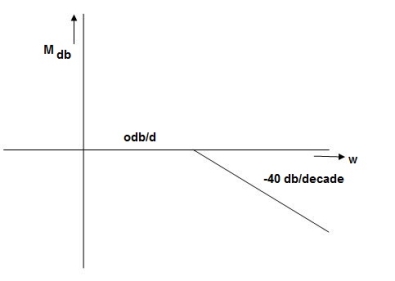
Fig 11 Magnitude Plot
Max error at MdB = -20 log10 For MdB = -20 log10
Completely the error depends upon the value of The maximum error will be MdB = -20 log10 M = -20 log10
M = - = Mr = MdB = -20 log10 MdB = -20 log10
Mr = |


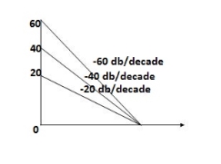
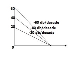
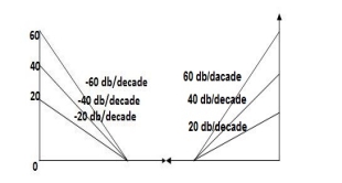
Type of system | Initial slope | Intersection |
0 | 0 dB/decade | Parallel to 0 axis |
1 | -20 dB/decade | =K1 |
2 | -40 dB/decade | =K1/2 |
3 | -60 dB/decade | =K1/3 |
. | . | 1 |
. | . | 1 |
. | . | 1 |
N | -20N dB/decade | =K1/N |
Stability Condition in Bode Plot :
The frequency at which the bode plot culls the 0db axis is called as Gain Cross Over Frequency.
|
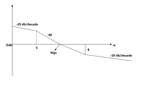
Fig 12 Gain cross over frequency
- Phase Cross Over Frequency
The Frequency at which the phase plot culls the -1800 axis.
|
Fig 13 Phase Margin and Gain Margin
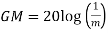
GM=MdB= -20 log [ G (jw)]
 .:
.: 
 .:
.: 
1) When gain cross over frequency is smaller than phase curves over frequency the system is stable and vice versa.
Key takeaways
- More the difference b/WPC and WGC core are the stability of system
- If GM is below 0dB axis than take ilb +ve and stable. if GM above 0dB axis, that is take -ve
- GM= ODB - 20 log M
- The IM should also lie above -1800 for making the system (i.e pm=+ve
- For a stable system GM and PM should be -ve
- GM and PM both should be +ve more the value of GM and PM more the system is stable.
- If Wpc and Wgc are in same line Wpc= Wgc than system is marginally stable as we get GM=0dB.
Sketching of Bode Plot:
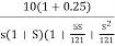
Q.1 sketch the bode plot for transfer function
G(S) =
G(j This is type 0 system. so initial slope is 0 dB decade. The starting point is given as 20 log10 K = 20 log10 1000 = 60 dB Corner frequency
Slope after 2. For phase plot
For phase plot
100 -900 200 -9.450 300 -104.80 400 -110.360 500 -115.420 600 -120.00 700 -124.170 800 -127.940 900 -131.350 1000 -134.420
|


The plot is shown in figure 14
|
|
|
|
Fig 14 Magnitude Plot for G(S) = 
Q.2 For the given transfer function determine
G(S) = Gain cross over frequency phase cross over frequency phase mergence and gain margin Initial slope = 1 N = 1 , (K)1/N = 2 K = 2 Corner frequency
1 -119.430 5 -172.230 10 -195.250 15 -209.270 20 -219.30 25 -226.760 30 -232.490 35 -236.980 40 -240.570 45 -243.490 50 -245.910 Finding M = 4 =
Let X3 (6.25 X1 = 2.46 X2 = -399.9 X3 = -6.50 For x1 = 2.46
for phase margin PM = 1800 -
= -164.50 PM = 1800 - 164.50 = 15.50 For phase cross over frequency (
-1800 = -900 – tan-1 (0.5 -900 – tan-1 (0.5 Taking than on both sides Tan 900 = tan-1 Let tan-1 0.5
1 =0.5
|


the plot is shown in figure 15.
|
|
|
|
Fig 15 Magnitude Plot G(S) = 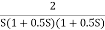
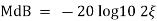
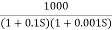
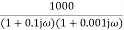
Q3. For the given transfer function
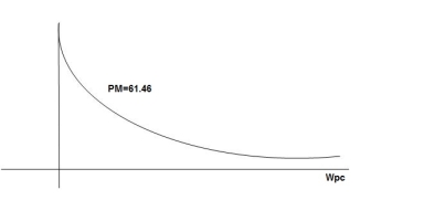
G(S) = Plot the rode plot find PM and GM T1 = 0.5 Zero so, slope (20 dB/decade) T2 = 0.2 Pole , so slope (-20 dB/decade) T3 = 0.1 = T4 = 0.1
Phase plot
500 -177.30 1000 -178.60 1500 -179.10 2000 -179.40 2500 -179.50 3000 -179.530 3500 -179.60 GM = 00 PM = 61.460
|


The plot is shown in figure 16
|
|
|
|
|
Fig 16 Magnitude and phase Plot for
G(S) = 
Q 4. For the given transfer function plot the bode plot (magnitude plot)
G(S) = Given transfer function G(S) = Converting above transfer function to standard from G(S) = =
T1 = T2 = 1 , 4. Initial slope will cut zero dB axis at (K)1/N = 10 i.e 5. finding T(S) = T(S)= Comparing with standard second order system equation S2+2
5. Maximum error M = -20 log 2 = +6.5 dB 6. As K = 10, so whole plot will shift by 20 log 10 10 = 20 dB
|


The plot is shown in figure 17
|
|
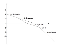
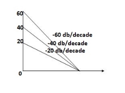
Fig 17 Magnitude Plot for G(S) = 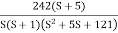
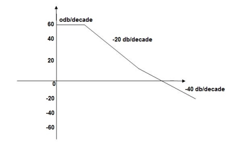
Q5. For the given plot determine the transfer function.
|
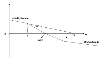
Fig 18 Magnitude Plot
From figure 18 we can conclude that
|


If the transfer function of a given system is not known than by the use of bode plot, we can determine the transfer function. The following steps should be followed
i) The experimental values of magnitude and phase plot should be plotted on the semi-log paper first.
ii) Then asymptotes are drawn which are the curves drawn by making sure that the slope of these asymptotes are multiples of ±20db/decade.
iii) The corner frequencies are adjusted such that the corner frequency on the asymptotic plot varies the actual plot by amount which can be corrected.
iv) If slope of magnitude curve obtained changes by -20db/decade at say  =
=  1. This means that 1/(1+j
 /
/ n)m exists in the transfer function which are poles of the system.
v) If slope changes by +20db/decade at  =
=  2. This means that (1+j
 /
/ n)m exists in the transfer function which are the zeros of the system.
vi) If slope changes by -40db/decade at  =
=  2 than it indicates double pole or pair of complex conjugate poles.
vii) If error between the asymptotic plot and actual plot is -6db then 1/(1+j /
/ n)2 is present and if error is +6db than a quadratic factor 1/[1+j2
 (
( /
/ 3) + (j
 /
/ 3)2] is present.
viii) At lower frequencies the plot is dominated by K/(j )r. Normally r has the values of 0,1 or 2. For type 0 k is given by K=1/20 log-1x
20logK = x.
ix) If the low frequency asymptote has slope -20db/decade then factor K/j in the transfer function for type-1.
x) For low asymptote has a slope of -40db/decade then the transfer function has term (K/j )2, then the plot intersects the0-db axis at
  .
.
xi) Now the phase plot is constructed as we now have the transfer function from the magnitude plot.
1) The more the value of gain margin more is the stability.
2) The more the value of phase margin more is the stability.
3) The gain cross over frequency, phase cross over frequency is used in determining the stability of system.
4) The frequency at which the two asymptotes cuts or meet each other is known as break frequency or corner frequency.
Phase – Lead Compensation:
The phase of output voltage leads the phase of input voltage for the applied sinusoidal input. The circuit diagram is shown below. The transfer function is given as,
|
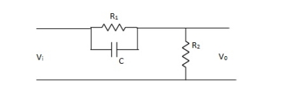
Fig 19 Phase Lead Compensation
Vo/Vi = α(1 + ST)/(1 + S α T) Where, α = R2/R1 + R2 and α< 1 T = R1C w = 1/T lower corner frequency due to zero. w = 1/ αT upper corner frequency due to pole. Mid frequency is given as, wm = 1/T√ α The maximum phase lead angle is φm Φm = tan-1(1- α)/2√α = Sin-11- α/1 + α |
Phase Lag Compensation:
|
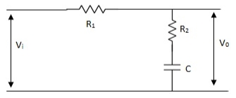
Fig 20 Phase Lag Compensation
Vo/Vi = 1 + ST/1 + SβT Where, β = R1 + R2/R2, β> 1 T = R2C w = 1/T upper corner frequency due to zero w= 1/βT lower corner frequency due to pole The mid frequency wm, wm = 1/T√β The maximum phase lead angle Φm Φm = tan-11- β/2 √β = sin-11 – β/1 + β |
Phase Lag-Lead Network:
To overcome the disadvantages of lead and lag compensation, they are used together. As lead compensation does not provide phase margin but has fast response and lag compensation stabilize the system but does not provide enough bandwidth.
|
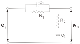
Fig 21 Lag-Lead Compensation
eo/ei = (1 + α ST1)/(1 + S T2)
T2)
Where, αT1 = R1C1
 T2= R2C2
we can say in the lag-lead compensation pole is more dominating than the zero and because of this lag-lead network may introduces positive phase angle to the system when connected in series.
Key takeaway
Phase Lead Network Phase Lag Network 1>. It is used to improve the 1>It is used to improve the transient response. Steady state response. 2>. It acts as a high pass filter. 2>It acts as a low pass filter. 3>. The system becomes fast as 3>The Bandwidth decreases Bandwidth increases as rise through rise time the speed Time decreases. is slow. 4>. As the circuit acts as 4>Signal to noise ratio is higher as it a differentiator, signal to acts as integrator. noise ratio is poor. 5>. Maximum peak overshoot 5>It reduces steady state error thus is reduced. improve the steady state accuracy
|
1. “Modern Control Engineering “, K. Ogata, Pearson Education Asia/
PHI, 4th Edition, 2002.
2. “Automatic Control Systems”, Benjamin C. Kuo, John Wiley India
Pvt. Ltd., 8th Edition, 2008.
3. “Feedback and Control System”, Joseph J Distefano III et al.,
Schaum’s Outlines, TMH, 2nd Edition 2007.
4. J. Nagarath and M.Gopal, “Control Systems Engineering”, New Age
International (P) Limited, Publishers, Fourth edition – 2005


