8.1 Concepts of state state variable and state models for electrical systems | unit 8 introduction to state variable analysis

UNIT - 8

Introduction to State variable analysis

8.1 Concepts of state, state variable and state models for electrical systems

8.1.1 Concepts of state, state variable

The state of a system is a minimal set of variables known as state variables. The knowledge of these variables at any instance of time together with the knowledge of the inputs for the same instance of time, determines the complete behaviour of the system. The fewer drawbacks in the transfer function method for representing any system led to the use of state variables in analysis of system. Few advantages are listed below:

The state space can be used for linear or nonlinear, time-variant or time-invariant systems.
It is easier to apply where Laplace transform cannot be applied.
The nth order differential equation can be expressed as 'n' equation of first order.
It is a time domain method.
As this is time domain method, therefore this method is suitable for digital computer computation.
On the basis of the given performance index, this system can be designed for an optimal condition.

Representation of state space: The system shown below has ‘m’ inputs, ‘p, outputs and ‘n’ number of state variables. The state equation gives us the relation between the state variables and the inputs.

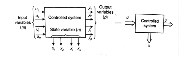
Fig 1 Representation of State space

So, the above system shown can be described through equations as

=f1 (x1, x2, xn, u1, u2………, um)

= f2 (x1, x2, xn, u1, u2………, um)

=f1 (x1, x2, xn, u1, u2………, um) (1)

The above set of equations can be represented as

=f(x(t),u(t)) (2)

As we are concerned for time invariant system, for which the term in (1) is linear combination of state variables and input. So,

(t)=2tx1+x2+u1+u2 (3)

=a11x1(t)+a12x2(t)+…a1nxn(t)+b11u1(t)+b12u2(t)+…….+b1mum(t)

=a21x1(t)+a22x2(t)+…a2nxn(t)+b21u1(t)+b22u2(t)+…….+b2mum(t)

=an1x1(t)+an2x2(t)+…annxn(t)+bn1u1(t)+bn2u2(t)+…….+bnmum(t)

The above equation can be represented in matrix form as given below

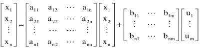
(4)

The above coefficients aij and bji in equation (4) can be written in vector matrix form as

=Ax(t)+Bu(t) (5)

The output of the system can be represented by linear combination of state variables and inputs.

y1=c11x1(t)+c12x2(t)+…….+c1nxn+d11u1+………..+d1mum

y2=c21x1(t)+c22x2(t)+…….+c2nxn+d21u1+………..+d2mum

yr=cr1x1(t)+cr2x2(t)+…….+crnxn+dr1u1+………..+drmum (6)

The equation (6) can be represented in matrix form as 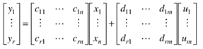(7)

Where coefficients cij and dji are constants. The output equation is given as

Y=CX+DU (8)

Key takeaway

The state equation is given as =Ax(t)+Bu(t)
The output equation is given as Y=CX+DU

8.1.2 State models for electrical systems

The state variables selected here are the physical quantities of the system, which can be measured. The selection of these variables can be directly related to the physical system because the solution of state equation is related to the time variation of the system variables.

The number of energy storing elements in any system is equal to the number of state variables. Below shown are few electrical circuits, just to brush up the concept of energy storing elements and state variable relation.

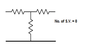
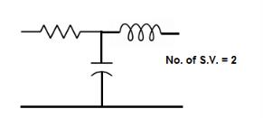
Fig 2 Electrical Circuits with energy storing elements

Now calculating the state equation and output equation for state variable analysis.

State Equation and Output equation:

Number of output=Number of output equation

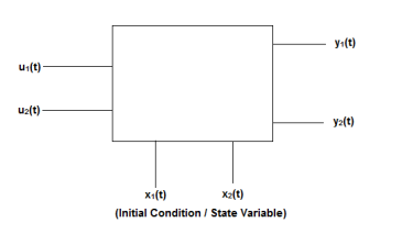
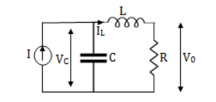
Fig 3 State Model

Considering multiple input and multiple output system, with two inputs u1(t)and u2(t), and two outputs y1(t) and y2(t) respectively.

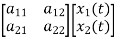
y1(t)=c11x1(t)+c12x2(t)+d11u1(t)+d12u2(t)

y2(t)=c21x1(t)+c22x2(t)+d21u1(t)+d22u2(t)

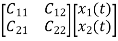
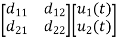
The output equation is given as

Y(t)=CX(t)+DU(t)

Y(t)= X(t)=

C= D=

U(t)=

# Now finding State Equation

Number of energy storing elements= Number of state variables

==a11x1(t)+a12x2(t)+b11u1(t)+b12u2(t)

==a21x1(t)+a22x2(t)+b21u1(t)+b22u2(t)

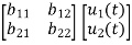
The state equation is then given as

=Ax(t)+Bu(t)

Key takeaways

The number of energies storing element= Number of state variables
We should always take voltage across the inductor L, and current through capacitor C.

Question: Obtatin the state space representation for the given electircal system

Solution: The state model is given as

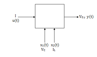
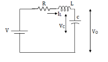
Fig 4 State Model

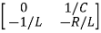
The state model shows that there are two energy storing elements L, C. As we already know that Number of state variables is equal to the number of energy storing elements.Hence we have two state variables[x1(t) and x2(t)]. We have one output V0(taken across capacitor) and input u(t).

The output equation is then given as

Y(t)=CX(t)+DU(t)

V0=Vc= x1(t) ….(a)

Hence output equation becomes

V0= x1(t)

y(t)=[1 0]+[0]u(t)

so, C=[1 0] D=[0]

Now writing the state equation

=Ax(t)+Bu(t)

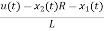
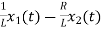
For that applying KVL in the above circuit

V=ILR+L+Vc

State Equation is =Ax(t)+Bu(t)

x1(t)=Vc

IL=C

=(1/C) x2(t) ……….(b)

VL=L

==VL/L

From KVL

L=VL=V-ILR-VC

= …………….(c)

From equation (b) and (c)

= [0 1/c]+ [0 0]u(t)

=[-1/L -R/L] + [1/L 0]

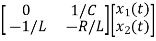
Now writing the state equation

=Ax(t)+Bu(t)

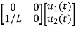
Hence A= B=

Question: Obtatin the state space representation for the given electircal system

Solution: The state model shows that there are two energy storing elements L, C. As we already know that Number of state variables is equal to the number of energy storing elements.Hence we have two state variables[x1(t) and x2(t)]. We have one output V0(taken across capacitor) and input u(t).

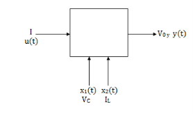
Fig 5 State Model

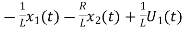
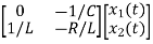
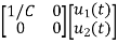
Here output is V0. But from above electrical circuit V0=ILR

V0=x2(t)R

y(t)= V0= [0 R] + [0] u(t)

The output equation is given as

Y(t)=CX(t)+DU(t)

C=[0 R] D=[0]

Now finding state equation,we apply KCL in the given electrical circuit

I=IC+IL

But I-IL=IC

=x2(t)+ ……..(a)

=[0 1/C]+ [1/C 0] …….(b)

Applying KVL in the given electrical circuit we get

VC=VL+ILR

VC-ILR=VL=L

=[1/L -R/L] + [0] u(t) ………….(c)

From equation (b) and (c) we have

Now writing the state equation

=Ax(t)+Bu(t)

Hence A= B=

Note: We should always take voltage across the inductor L, and current through capacitor C.

8.2 Solution of state equations

Solution of homogeneous state equations

The first order differential equation is given as

=ax x(0)=x0

x(t)=x0=

Consider state equation

=Ax(t); x(0)=x0

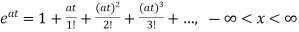
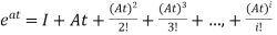
The solution will be of the form

x(t)=a0+a1t+a2t2+a3t3+….+aiti

substituting value in above equation

a1+2a2t2+3a3t3+……….=A[a0+a1t+a2t2+a3t3+….+aiti]

a1=Aa0

a2=Aa1=A2a0

ai=Aia0

Solution for x(t) will be

x(t)=[I+At+A2t2+………+Aiti]x0

The matrix exponential form can be written as

The solution x(t) will be x(t)=x0

=Ax(t)+Bu(t) and x(0)=x0

- Ax(t)=Bu(t)

Multiplying both sides by

[ - Ax(t)]==Bu(t)

Integrating both sides w.r.t t we get

= d

Multiplying both sides by

x(t)=x(0)+d

x(0) is called as Homogeneous solution

dis the Forced solution

At t=t0

x(t)=x(t0)+d

The above equation is the required solution

Solution of non-homogeneous state equation

Let the scalar state equation be

=ax+bu

-ax=bu

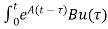
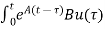
Multiplying both sides by e-at

x(t) = eat x(0) +d

Then for non-homogeneous state equation

=Ax+Bu

The solution x(t) can be given as

x(t) = eAt x(0) +d

The above equation is the required solution.

Key takeaway

Then for non-homogeneous state equation

=Ax+Bu

2. The solution x(t) can be given as

x(t) = eAt x(0) +d

The above equation is the required solution.

3. Then for homogeneous state equation

x(t)=x(t0)+d

The above equation is the required solution

Reference

1. “Modern Control Engineering “, K. Ogata, Pearson Education Asia/

PHI, 4th Edition, 2002.

2. “Automatic Control Systems”, Benjamin C. Kuo, John Wiley India

Pvt. Ltd., 8th Edition, 2008.

3. “Feedback and Control System”, Joseph J Distefano III et al.,

Schaum’s Outlines, TMH, 2nd Edition 2007.

4. J. Nagarath and M. Gopal, “Control Systems Engineering”, New Age

International (P) Limited, Publishers, Fourth edition – 2005

Sign Up

Index

Notes

Highlighted

Underlined

Browse by Topics

Notes

Highlighted

Underlined