BUSINESS STATISTICS

BUSINESS STATISTICS

BUSINESS STATISTICS

UNIT 1V

Moments, Skewness and Kurtosis

QUESTION AND ANSWERS

1.     Define moments?

ANS

Moments are a set of statistical parameters to measure a distribution. Four moments are commonly used:

•         1st moment - Mean (describes central value)

•         2nd moment - Variance (describes dispersion)

•         3rd moment - Skewness (describes asymmetry)

•         4th moment - Kurtosis (describes peakedness)

2.     What are raw moments and central moments ?

ANS

The n-th moment about zero of a probability density function f(x) is the expected value of Xn and is called a raw moment or crude moment. The moments about its mean μ are called central moments; these describe the shape of the function, independently of translation.

A moment  of a probability function  taken about 0,

			(1)
			(2)

The raw moments  (sometimes also called "crude moments") can be expressed as terms of the central moments  (i.e., those taken about the mean ) using the inverse binomial transform

(3)

With  and  (Papoulis 1984, p. 146). The first few values are therefore

			(4)
			(5)
			(6)
			(7)

The raw moments  can also be expressed in terms of the cumulates  by exponentiating both sides of the series

(8)

Where  is the characteristic function, to obtain

(9)

The first few terms are then given by

			(10)
			(11)
			(12)
			(13)
			(14)

The raw moment of a multivariate probability function  can be similarly defined as

(15)

Therefore,

(16)

The multivariate raw moments can be expressed in terms of the multivariate cumulants. For example,

			(17)
			(18)

In probability theory and statistics, a central moment is a moment of a probability distribution of a random variable about the random variable's mean; that is, it is the expected value of a specified integer power of the deviation of the random variable from the mean. The various moments form one set of values by which the properties of a probability distribution can be usefully characterized. Central moments are used in preference to ordinary moments, computed in terms of deviations from the mean instead of from zero, because the higher-order central moments relate only to the spread and shape of the distribution, rather than also to its location.

Sets of central moments can be defined for both univariate and multivariate distributions.

ANS

Skewness is the measure of the asymmetry of an ideally symmetric probability distribution and is given by the third standardized moment. If that sounds way too complex, don’t worry! Let me break it down for you.

In simple words, skewness is the measure of how much the probability distribution of a random variable deviates from the normal distribution. Now, you might be thinking – why am I talking about normal distribution here?

Well, the normal distribution is the probability distribution without any skewness. You can look at the image below which shows symmetrical distribution that’s basically a normal distribution and you can see that it is symmetrical on both sides of the dashed line. Apart from this, there are two types of skewness:

• Positive Skewness
• Negative Skewness

ANS

Skewness is a measure of symmetry or lack of symmetry in a distribution. A distribution is symmetric if it looks same both its left and right side. The skewness for normal distribution is Zero. Negative values for skewness indicate that the data are skewed left and positive values for skewness indicate that the data are skewed right. For small data sets, this measure is unreliable. The below diagram shows how a normal distribution curve looks like in different situation of skewness:

The formula for measuring Coefficient of Skewness as given by Karl Pearson is as under:

=

Where, = Karl Pearson’s Coefficient of Skewness

= Standard Deviation

The formula for measuring Co-efficient of Skewness as given by Bowley is as under:

Example 1: From the following data, calculate Karl Pearson’s Co-efficient of Skewness:

Mean = 16, Mode = 38, Standard Deviation = 5

Solution: We know that

=

=

= -4.4

Example 2 – Below are the data of hours spent watching television by the 220 students. Calculate Karl Pearsons Co-efficient of Skewness.

Solution:

Hours	No. Of students	x	Fx	X – x	(x – x ) 2	F (x – x ) 2
10 – 14	2	12	24	-17.82	317.49	634.98
15 – 19	12	17	204	-12.82	164.31	1971.67
20 – 24	23	22	506	-7.82	61.12	1405.85
25 – 29	60	27	1620	-2.82	7.94	476.53
30 – 34	77	32	2464	2.18	4.76	366.55
35 – 39	38	37	1406	7.18	51.58	1959.98
40 - 44	8	42	336	12.18	148.40	1187.17
	220		6560			8002.73

Mean = 6560/220 = 29.82

SD = √8002.73/220 = 6.03

Mode = L1 + (L2 – L1)   d1

                          d1 +d2

Here modal class is 30 – 34 (Since the frequency is highest)

L1 = 30, L2 = 34, d1 = 17, d2 = 39

Mode = 30 + (34 – 30)   17

                          17 + 39

Mode = 30 + x 17

          = 30 + 1.21

          = 31.21

Therefore, Co-efficient of Skewness

=

       =

          = - 0.23

Example 3: Calculate Bowley’s Coefficient of Skewness from the following test scores:

Solution:

First quartile (Q1)

Qi= [i * (n + 1) /4] th observation

Q1= [1 * (8 + 1) /4] th observation

Q1 = 2.25 th observation

Thus, 2.25 th observation lies between the 2nd and 3rd value in the ordered group, between frequency 17 and 26

First quartile (Q1) is calculated as

Q1 = 2nd observation +0.75 * (3rd observation - 2nd observation)

Q1 = 17 + 0.75 * (26 – 17) = 23.75

Second quartile()

Q2= [2 * (8 + 1) /4] th observation

Q2 =   4.5th Observation

So, 4.5th observation lies between 4th and 5th value in ordered group, between frequency 27 and 30.

Hence Q2 = 4th observation + 0.50 * (5th observation – 6th observation)

Q2 = 27 + 0.50 * (30 – 27) = 28.5

Third quartile (Q3)

Qi= [i * (n + 1) /4] th observation

Q3= [3 * (8 + 1) /4] th observation

Q3 = 6.75 th observation

So, 6.75 th observation lies between the 6th and 7th value in the ordered group, between frequency 30 and 31

Third quartile (Q3) is calculated as

Q3 = 6th observation +0.25 * (7th observation – 6th observation)

Q3 = 30 + 0.25 * (31 – 30) = 30.25

Therefore, Bowley’s Coefficient of Skewness is calculated as under:

=

= = - 0.461

5.     What is Kurtosis?

ANS

Kurtosis is a statistical measure that defines how heavily the tails of a distribution differ from the tails of a normal distribution. In other words, kurtosis identifies whether the tails of a given distribution contain extreme values.

Along with skewness, kurtosis is an important descriptive statistic of data distribution. However, the two concepts must not be confused with each other. Skewness essentially measures the symmetry of the distribution, while kurtosis determines the heaviness of the distribution tails.

6.     What is Excess Kurtosis?

An excess kurtosis compares the  kurtosis of a distribution against the kurtosis of a normal distribution. The kurtosis of a normal distribution equals 3. Therefore, the excess kurtosis is found using the formula below:

Excess Kurtosis = Kurtosis – 3

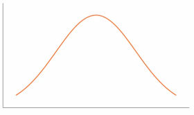
7.     What is Platykurtic ?

ANS

When the kurtosis < 0, shows a negative excess kurtosis, the frequencies throughout the curve are closer to be equal (i.e., the curve is flatter and wider)

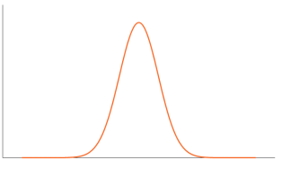
8.     What is Leptokurtic?

ANS

When the kurtosis > 0,indicates positive excess kurtosis,  there are high frequencies in only a small part of the curve (i.e., the curve is more peaked)

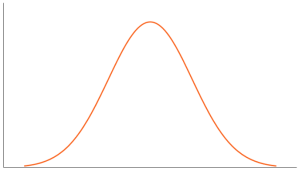
9.     What is Mesokurtic?

ANS

When the kurtosis = 0. Indicates excess kurtosis of zero or close to zero. It refers to the data flows in normal distribution.

10.  What are the formulas for calculating moments?

ANS

The formula for calculating moments is as follows:

1st moment =

2nd moment =

3rd moment  =

4th moment =