BUSINESS STATISTICS
BUSINESS STATISTICS
UNIT V
Correlation and Regression
QUESTION AND ANSWERS
- What is Scatter diagram?
ANS
The Scatter Diagram Method is the simplest method to study the correlation between two variables wherein the values for each pair of a variable is plotted on a graph in the form of dots thereby obtaining as many points as the number of observations. Then by looking at the scatter of several points, the degree of correlation is ascertained.
The degree to which the variables are related to each other depends on the manner in which the points are scattered over the chart. The more the points plotted are scattered over the chart, the lesser is the degree of correlation between the variables. The more the points plotted are closer to the line, the higher is the degree of correlation. The degree of correlation is denoted by “r”.
2. What are the different types of scatter diagram?
ANS
There are different types of scatter diagram depicting the type of correlation which may be as under:
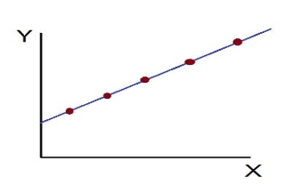
- Perfect Positive Correlation (r=+1): The correlation is said to be perfectly positive when all the points lie on the straight line rising from the lower left-hand corner to the upper right-hand corner.

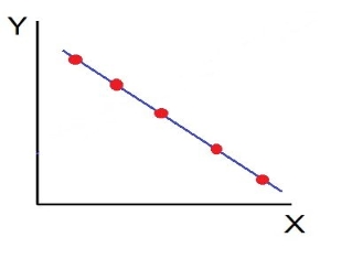
Ii. Perfect Negative Correlation (r=-1): When all the points lie on a straight line falling from the upper left-hand corner to the lower right-hand corner, the variables are said to be negatively correlated.
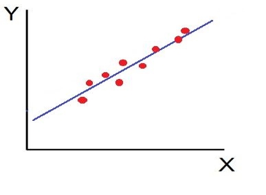
Iii. High Degree of +Ve Correlation (r= + High): The degree of correlation is high when the points plotted fall under the narrow band and is said to be positive when these show the rising tendency from the lower left-hand corner to the upper right-hand corner.
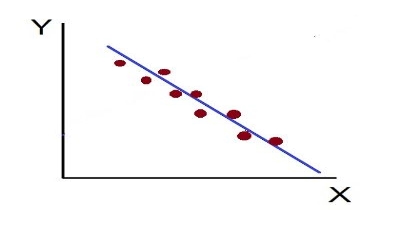
Iv. High Degree of –Ve Correlation (r= – High): The degree of negative correlation is high when the point plotted fall in the narrow band and show the declining tendency from the upper left-hand corner to the lower right-hand corner.
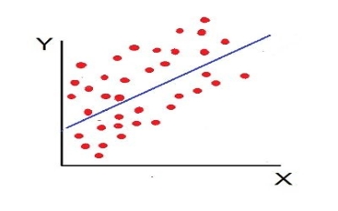
v. Low degree of +Ve Correlation (r= + Low): The correlation between the variables is said to be low but positive when the points are highly scattered over the graph and show a rising tendency from the lower left-hand corner to the upper right-hand corner.
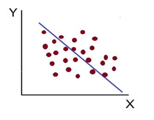
Vi. Low Degree of –Ve Correlation (r= + Low): The degree of correlation is low and negative when the points are scattered over the graph and the show the falling tendency from the upper left-hand corner to the lower right-hand corner.
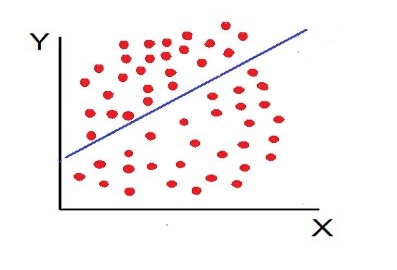
Vii. No Correlation (r= 0): The variable is said to be unrelated when the points are haphazardly scattered over the graph and do not show any specific pattern. Here the correlation is absent and hence r = 0
Thus, the scatter diagram method is the simplest device to study the degree of relationship between the variables by plotting the dots for each pair of variable values given. The chart on which the dots are plotted is also called as a Dotogram.
3. What is two way tables?
ANS
Two-way tables organize data based on two categorical variables.
Two way frequency tables
Two-way frequency tables show how many data points fit in each category. A two-way table (also called a contingency table) is a useful tool for examining relationships between categorical variables. The entries in the cells of a two-way table can be frequency counts or relative frequencies (just like a one-way table ).
| Dance | Sports | TV | Total |
Men | 2 | 10 | 8 | 20 |
Women | 16 | 6 | 8 | 30 |
Total | 18 | 16 | 16 | 50 |
Above, a two-way table shows the favorite leisure activities for 50 adults - 20 men and 30 women. Because entries in the table are frequency counts, the table is a frequency table.
Here's another example:
Preference | Male | Female |
Prefers dogs | 363636 | 222222 |
Prefers cats | 888 | 262626 |
No preference | 222 | 666 |
The columns of the table tell us whether the student is a male or a female. The rows of the table tell us whether the student prefers dogs, cats, or doesn't have a preference.
Each cell tells us the number (or frequency) of students. For example, the 363636 is in the male column and the prefers dogs row. This tells us that there are 363636 males who preferred dogs in this dataset.
Notice that there are two variables—gender and preference—this is where the two in two-way frequency table comes from.
4. What is conditional distribution?
ANS
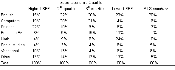
A conditional distribution is a probability distribution for a sub-population. In other words, it shows the probability that a randomly selected item in a sub-population has a characteristic you’re interested in. For example, if you are studying eye colors (the population) you might want to know how many people have blue eyes (the sub-population). Conditional distributions are easier to find with the help of a table.
The following table shows how computer use differs across socio-economic backgrounds. The table shows the “big picture” across all subjects for the entire sample. SES in the table stands for socio-economic status.
5. What is marginal distribution?
ANS
Definition of a marginal distribution = If X and Y are discrete random variables and f (x,y) is the value of their joint probability distribution at (x,y), the functions given by:
g(x) = Σy f (x,y) and h(y) = Σx f (x,y) are the marginal distributions of X and Y , respectively.
A marginal distribution gets its name because it appears in the margins of a probability distribution table.

Of course, it’s not quite as simple as that. You can’t just look at any old frequency distribution table and say that the last column (or row) is a “marginal distribution.” Marginal distributions follow a couple of rules:
- The distribution must be from bivariate data. Bivariate is just another way of saying “two variables,” like X and Y. In the table above, the random variables i and j are coming from the roll of two dice.
- A marginal distribution is where you are only interested in one of the random variables. In other words, either X or Y. If you look at the probability table above, the sum probabilities of one variable are listed in the bottom row and the other sum probabilities are listed in the right column. So this table has two marginal distributions.
6. What is Karl Pearson’s Coefficient of Correlation?
ANS
Karl Pearson’s Coefficient of Correlation is widely used mathematical method is used to calculate the degree and direction of the relationship between linear related variables. The coefficient of correlation is denoted by “r”.
Direct method
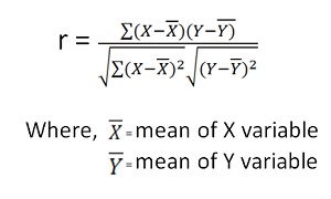
Shortcut method –


The value of the coefficient of correlation (r) always lies between ±1. Such as:
- r=+1, perfect positive correlation
- r=-1, perfect negative correlation
- r=0, no correlation
7. Compute Pearson’s coefficient of correlation between advertisement cost and sales as per the data given below:
Advertisement cost | 39 | 65 | 62 | 90 | 82 | 75 | 25 | 98 | 36 | 78 |
Sales | 47 | 53 | 58 | 86 | 62 | 68 | 60 | 91 | 51 | 84 |
ANS
X | Y |
|
|
|
|
 |
39 | 47 | -26 | 676 | -19 | 361 | 494 |
65 | 53 | 0 | 0 | -13 | 169 | 0 |
62 | 58 | -3 | 9 | -8 | 64 | 24 |
90 | 86 | 25 | 625 | 20 | 400 | 500 |
82 | 62 | 17 | 289 | -4 | 16 | -68 |
75 | 68 | 10 | 100 | 2 | 4 | 20 |
25 | 60 | -40 | 1600 | -6 | 36 | 240 |
98 | 91 | 33 | 1089 | 25 | 625 | 825 |
36 | 51 | -29 | 841 | -15 | 225 | 435 |
78 | 84 | 13 | 169 | 18 | 324 | 234 |
650 | 660 |
| 5398 |
| 2224 | 2704 |
|
|
|
|
|
|
|

r = (2704)/√5398 √2224 = (2704)/(73.2*47.15) = 0.78
Thus Correlation coefficient is positively correlated
8. Compute correlation coefficient from the following data
Hours of sleep (X) | Test scores (Y) |
8 | 81 |
8 | 80 |
6 | 75 |
5 | 65 |
7 | 91 |
6 | 80 |
ANS
X | Y |
|
|
|
|
 |
8 | 81 | 1.3 | 1.8 | 2.3 | 5.4 | 3.1 |
8 | 80 | 1.3 | 1.8 | 1.3 | 1.8 | 1.8 |
6 | 75 | -0.7 | 0.4 | -3.7 | 13.4 | 2.4 |
5 | 65 | -1.7 | 2.8 | -13.7 | 186.8 | 22.8 |
7 | 91 | 0.3 | 0.1 | 12.3 | 152.1 | 4.1 |
6 | 80 | -0.7 | 0.4 | 1.3 | 1.8 | -0.9 |
40 | 472 |
| 7 |
| 361 | 33 |

X = 40/6 =6.7

Y = 472/6 = 78.7

r = (33)/√7 √361 = (33)/(2.64*19) = 0.66
Thus Correlation coefficient is positively correlated
9. Calculate coefficient of correlation between X and Y series using Karl Pearson shortcut method
X | 14 | 12 | 14 | 16 | 16 | 17 | 16 | 15 |
Y | 13 | 11 | 10 | 15 | 15 | 9 | 14 | 17 |
ANS
Let assumed mean for X = 15, assumed mean for Y = 14
X | Y | Dx | Dx2 | Dy | Dy2 | Dxdy |
14 | 13 | -1.0 | 1.0 | -1.0 | 1.0 | 1.0 |
12 | 11 | -3.0 | 9.0 | -3.0 | 9.0 | 9.0 |
14 | 10 | -1.0 | 1.0 | -4.0 | 16.0 | 4.0 |
16 | 15 | 1.0 | 1.0 | 1.0 | 1.0 | 1.0 |
16 | 15 | 1.0 | 1.0 | 1.0 | 1.0 | 1.0 |
17 | 9 | 2.0 | 4.0 | -5.0 | 25.0 | -10.0 |
16 | 14 | 1 | 1 | 0 | 0 | 0 |
15 | 17 | 0 | 0 | 3 | 9 | 0 |
120 | 104 | 0 | 18 | -8 | 62 | 6 |

 r = 8 *6 – (0)*(-8)
√8*18-(0)2 √8*62 – (-8)2
r = 48/√144*√432 = 0.19
10. Calculate coefficient of correlation between X and Y series using Karl Pearson shortcut method
X | 1800 | 1900 | 2000 | 2100 | 2200 | 2300 | 2400 | 2500 | 2600 |
F | 5 | 5 | 6 | 9 | 7 | 8 | 6 | 8 | 9 |
ANS
Assumed mean of X and Y is 2200, 6
X | Y | Dx | Dx (i=100) | Dx2 | Dy | Dy2 | Dxdy |
1800 | 5 | -400 | -4 | 16 | -1.0 | 1.0 | 4.0 |
1900 | 5 | -300 | -3 | 9 | -1.0 | 1.0 | 3.0 |
2000 | 6 | -200 | -2 | 4 | 0.0 | 0.0 | 0.0 |
2100 | 9 | -100 | -1 | 1 | 3.0 | 9.0 | -3.0 |
2200 | 7 | 0 | 0 | 0 | 1.0 | 1.0 | 0.0 |
2300 | 8 | 100 | 1 | 1 | 2.0 | 4.0 | 2.0 |
2400 | 6 | 200 | 2 | 4 | 0 | 0 | 0.0 |
2500 | 8 | 300 | 3 | 9 | 2 | 4 | 6.0 |
2600 | 9 | 400 | 4 | 16 | 3 | 9 | 12.0 |
|
|
|
|
|
|
|
|
|
|
| 0 | 60 | 9 | 29 | 24 |
Note – we can also proceed dividing x/100
 r = (9)(24) – (0)(9)
√9*60-(0)2 √9*29– (9)2
r = 0.69
11. Calculate coefficient of correlation between X and Y series using Karl Pearson shortcut method
X | 28 | 45 | 40 | 38 | 35 | 33 | 40 | 32 | 36 | 33 |
Y | 23 | 34 | 33 | 34 | 30 | 26 | 28 | 31 | 36 | 35 |
ANS
X | Y |
|
|
|
|
 |
28 | 23 | -8 | 64 | -8.0 | 64.0 | 64.0 |
45 | 34 | 9 | 81 | 3.0 | 9.0 | 27.0 |
40 | 33 | 4 | 16 | 2.0 | 4.0 | 8.0 |
38 | 34 | 2 | 4 | 3.0 | 9.0 | 6.0 |
35 | 30 | -1 | 1 | -1.0 | 1.0 | 1.0 |
33 | 26 | -3 | 9 | -5.0 | 25.0 | 15.0 |
40 | 28 | 4 | 16 | -3 | 9 | -12.0 |
32 | 31 | -4 | 16 | 0 | 0 | 0.0 |
36 | 36 | 0 | 0 | 5 | 25 | 0.0 |
33 | 35 | -3 | 9 | 4 | 16 | -12 |
360 | 310 | 0 | 216 | 0 | 162 | 97 |

 X = 360/10 = 36
Y = 310/10 = 31

r = 97/(√216 √162 = 0.51
12. What are Simple regression lines and properties?
ANS
It is a mathematical method and with it gives a fitted trend line for the set of data in such a manner that the following two conditions are satisfied.
- The sum of the deviations of the actual values of Y and the computed values of Y is zero.
- The sum of the squares of the deviations of the actual values and the computed values is least.
This method gives the line which is the line of best fit. This method is applicable to give results either to fit a straight-line trend or a parabolic trend.
The method of least squares as studied in time series analysis is used to find the trend line of best fit to a time series data.
13. What is Spearman’s rank correlation?
ANS
Spearman’s Rank Correlation Coefficient - The Spearman’s Rank Correlation Coefficient is the non-parametric statistical measure used to study the strength of association between the two ranked variables. This method is used for ordinal set of numbers, which can be arranged in order.

Where, P = Rank coefficient of correlation
D = Difference of ranks
N = Number of Observations
The Spearman’s Rank Correlation coefficient lies between +1 to -1.
- +1 indicates perfect association of rank
- 0 indicates no association between the rank
- -1 indicates perfect negative association between the ranks
When ranks are not given - Rank by taking the highest value or the lowest value as 1
Equal Ranks or Tie in Ranks – in this case ranks are assigned on an average basis. For ex – if three students score of 5, at 5th, 6th, 7th ranks ach one of them will be assigned a rank of 5 + 6 + 7/3= 6.
If two individual ranked equal at third position, then the rank is Calculate as (3+4)/2 = 3.5
14. Find spearman’s rank correlation from the following data :
Test 1 | 8 | 7 | 9 | 5 | 1 |
Test 2 | 10 | 8 | 7 | 4 | 5 |
ANS
Here, highest value is taken as 1
Test 1 | Test 2 | Rank T1 | Rank T2 | d | d2 |
8 | 10 | 2 | 1 | 1 | 1 |
7 | 8 | 3 | 2 | 1 | 1 |
9 | 7 | 1 | 3 | -2 | 4 |
5 | 4 | 4 | 5 | -1 | 1 |
1 | 5 | 5 | 4 | 1 | 1 |
|
|
|
|
| 8 |

p = 1 – (6*8)/5(52 – 1) = 0.60
15. Calculate Spearman rank-order correlation
English | 56 | 75 | 45 | 71 | 62 | 64 | 58 | 80 | 76 | 61 |
Maths | 66 | 70 | 40 | 60 | 65 | 56 | 59 | 77 | 67 | 63 |
ANS
Rank by taking the highest value or the lowest value as 1.
Here, highest value is taken as 1
English | Maths | Rank (English) | Rank (Math) | d | d2 |
56 | 66 | 9 | 4 | 5 | 25 |
75 | 70 | 3 | 2 | 1 | 1 |
45 | 40 | 10 | 10 | 0 | 0 |
71 | 60 | 4 | 7 | -3 | 9 |
62 | 65 | 6 | 5 | 1 | 1 |
64 | 56 | 5 | 9 | -4 | 16 |
58 | 59 | 8 | 8 | 0 | 0 |
80 | 77 | 1 | 1 | 0 | 0 |
76 | 67 | 2 | 3 | -1 | 1 |
61 | 63 | 7 | 6 | 1 | 1 |
|
|
|
|
| 54 |

 p = 1-(6*54)
10(102-1)
p = 0.67
Therefore this indicates a strong positive relationship between the rank’s individuals obtained in the math and English exam.
16. Find Spearman's rank correlation coefficient between X and Y for this set of data:
X | 13 | 20 | 22 | 18 | 19 | 11 | 10 | 15 |
Y | 17 | 19 | 23 | 16 | 20 | 10 | 11 | 18 |
ANS
X | Y | Rank X | Rank Y | d | d2 |
13 | 17 | 3 | 4 | -1 | 1 |
20 | 19 | 7 | 6 | 1 | 1 |
22 | 23 | 8 | 8 | 0 | 0 |
18 | 16 | 5 | 3 | 2 | 2 |
19 | 20 | 6 | 7 | -1 | 1 |
11 | 10 | 2 | 1 | 1 | 1 |
10 | 11 | 1 | 2 | -1 | 1 |
15 | 18 | 4 | 5 | -1 | 1 |
|
|
|
|
| 8 |
p =

 p = 1 – 6*8/8(82 – 1) = 1 – 48 = 0.90 504
17. Calculation of equal ranks or tie ranks
Find Spearman's rank correlation coefficient:
Commerce | 15 | 20 | 28 | 12 | 40 | 60 | 20 | 80 |
Science | 40 | 30 | 50 | 30 | 20 | 10 | 30 | 60 |
ANS
C | S | Rank C | Rank S | d | d2 |
15 | 40 | 2 | 6 | -4 | 16 |
20 | 30 | 3.5 | 4 | -0.5 | 0.25 |
28 | 50 | 5 | 7 | -2 | 4 |
12 | 30 | 1 | 4 | -3 | 9 |
40 | 20 | 6 | 2 | 4 | 16 |
60 | 10 | 7 | 1 | 6 | 36 |
20 | 30 | 3.5 | 4 | -0.5 | 0.25 |
80 | 60 | 8 | 8 | 0 | 0 |
|
|
|
|
| 81.5 |

p = 1 – (6*81.5)/8(82 – 1) = 0.02
18. Find Spearman's rank correlation coefficient:
X | 10 | 15 | 11 | 14 | 16 | 20 | 10 | 8 | 7 | 9 |
Y | 16 | 16 | 24 | 18 | 22 | 24 | 14 | 10 | 12 | 14 |
ANS
X | Y | Rank X | Rank Y | d | d2 |
10 | 16 | 6.5 | 5.5 | 1 | 1 |
15 | 16 | 3 | 5.5 | -2.5 | 6.25 |
11 | 24 | 5 | 1.5 | 3.5 | 12.25 |
14 | 18 | 4 | 4 | 0 | 0 |
16 | 22 | 2 | 3 | -1 | 1 |
20 | 24 | 1 | 1.5 | -0.5 | 0.25 |
10 | 14 | 6.5 | 7.5 | -1 | 1 |
8 | 10 | 9 | 10 | -1 | 1 |
7 | 12 | 10 | 9 | 1 | 1 |
9 | 14 | 8 | 7.5 | 0.5 | 0.25 |
|
|
|
|
| 24 |

p = 1 – (6*24)/10(102 – 1) = 0.85
The correlation between X and Y is positive and very high.
19. What are the coefficients of correlation ?
ANS
The value of the coefficient of correlation (r) always lies between ±1. Such as:
- r=+1, perfect positive correlation
- r=-1, perfect negative correlation
- r=0, no correlation
20. What is secured trend line?
Ans
The secular trend line (Y) is defined by the following equation:
Y = a + b X
Where, Y = predicted value of the dependent variable
a = Y-axis intercept i.e. the height of the line above origin (when X = 0, Y = a)
b = slope of the line (the rate of change in Y for a given change in X)
When b is positive the slope is upwards, when b is negative, the slope is downwards
X = independent variable (in this case it is time)
To estimate the constants a and b, the following two equations have to be solved simultaneously:
ΣY = na + b ΣX
ΣXY = aΣX + bΣX2
To simplify the calculations, if the midpoint of the time series is taken as origin, then the negative values in the first half of the series balance out the positive values in the second half so that ΣX = 0. In this case, the above two normal equations will be as follows:
ΣY = na
ΣXY = bΣX2
Logarithm y = aebx.
The equation is
y = aebx.
Taking log to the base e on both sides,
We get logy = loga + bx.
Which can be replaced as Y=A+BX,
Where Y = logy, A = loga, B = b and X = x.
21. Fit the straight line to the following data.
x | 1 | 2 | 3 | 4 | 5 |
y | 1 | 2 | 3 | 4 | 5 |
ANS
The normal equations are:
Σy = aΣx + nb
And
Σxy = aΣx2 + bΣx
Now,
x | y | x2 | Xy |
1 | 1 | 1 | 1 |
2 | 2 | 4 | 4 |
3 | 3 | 9 | 9 |
4 | 4 | 16 | 16 |
5 | 5 | 25 | 25 |
Σx = 15 | Σy = 15 | Σx2 = 55 | Σxy = 55 |
Substituting in the equations,
15 = 15a + 4b and 55 = 55a + 15b
Solving these two equations,
We get a=1 and b=0,
Therefore the required straight-line equation is y=x.
22. Fit the straight-line curve to the following data.
x | 75 | 80 | 93 | 65 | 87 | 71 | 98 | 68 | 84 | 77 |
y | 82 | 78 | 86 | 72 | 91 | 80 | 95 | 72 | 89 | 74 |
ANS
First drawing the table,
x | y | x2 | Xy |
75 | 82 | 5625 | 6150 |
80 | 78 | 6400 | 6240 |
93 | 86 | 8349 | 7998 |
65 | 72 | 4225 | 4680 |
87 | 91 | 7569 | 7917 |
71 | 80 | 5041 | 5680 |
98 | 95 | 9605 | 9310 |
68 | 72 | 4624 | 4896 |
84 | 89 | 7056 | 7476 |
77 | 74 | 5929 | 5698 |
798 | 819 | 64422 | 66045 |
The normal equation is:
Σy = aΣx + nb
and
Σxy = aΣx2 + bΣx.
Substituting the values, we get,
819 = 798a + 10b
66045 = 64422a + 798b
Solving, we get
a = 0.9288 and b = 7.78155
Therefore, the straight-line equation is:
y = 0.9288x + 7.78155.
23. Fit a second-degree parabola to the following data.
x | 1 | 2 | 3 | 4 | 5 | 6 | 7 | 8 | 9 |
y | 2 | 6 | 7 | 8 | 10 | 11 | 11 | 10 | 9 |
ANS
Here,
x | y | x2 | x3 | x4 | Xy | x2y |
1 | 2 | 1 | 1 | 1 | 2 | 2 |
2 | 6 | 4 | 8 | 16 | 12 | 24 |
3 | 7 | 9 | 27 | 81 | 21 | 63 |
4 | 8 | 16 | 64 | 256 | 32 | 128 |
5 | 10 | 25 | 125 | 625 | 50 | 250 |
8 | 11 | 36 | 216 | 1296 | 66 | 396 |
7 | 11 | 49 | 343 | 2401 | 77 | 539 |
8 | 10 | 64 | 512 | 4096 | 80 | 640 |
9 | 9 | 81 | 729 | 6561 | 81 | 729 |
45 | 74 | 285 | 2025 | 15333 | 421 | 2771 |
The normal equations are:
Σy = aΣx2 + b Σx + nc
Σxy = aΣx3 + bΣx2 +c Σx
Σx2y = aΣx4 + bΣx3 + cΣx2
Substituting the values, we get
74 = 285a + 45b + 9c
421 = 2025 a + 285 b + 45 c
2771 = 15333a + 2025 b + 285 c
Solving them, we get the second order equation which is,
y = -0.2673x2 + 3.5232x – 0.9286.


