Unit-10A

Biostatistics covering

Q1) What is Biostatistics and what is its main purpose?

A1)

Biostatistics is the development and application of statistical methods to a wide range of topics in biology. It encompasses the design of biological experiments, the collection and analysis of data from those experiments and the interpretation of the results.

Biostatistical modeling forms an important part of numerous modern biological theories. Genetics studies, since its beginning, used statistical concepts to understand observed experimental results. Some genetics scientists even contributed with statistical advances with the development of methods and tools. Gregor Mendel started the genetics studies investigating genetics segregation patterns in families of peas and used statistics to explain the collected data. In the early 1900s, after the rediscovery of Mendel's Mendelian inheritance work, there were gaps in understanding between genetics and evolutionary Darwinism. Francis Galton tried to expand Mendel's discoveries with human data and proposed a different model with fractions of the heredity coming from each ancestral composing an infinite series. He called this the theory of "Law of Ancestral Heredity". His ideas were strongly disagreed by William Bateson, who followed Mendel's conclusions that genetic inheritance were exclusively from the parents, half from each of them. This led to a vigorous debate between the biometricians, who supported Galton's ideas, as Walter Weldon, Arthur Dukinfield Darbishire and Karl Pearson, and Mendelians, who supported Bateson's (and Mendel's) ideas, such as Charles Davenport and Wilhelm Johannsen. Later, biometricians could not reproduce Galton conclusions in different experiments, and Mendel's ideas prevailed. By the 1930s, models built on statistical reasoning had helped to resolve these differences and to produce the neo-Darwinian modern evolutionary synthesis.

Q2) What is planning and research to solving the Biostatics terms?

A2)

Any research in life sciences is proposed to answer a scientific question we might have. To answer this question with a high certainty, we need accurate results. The correct definition of the main hypothesis and the research plan will reduce errors while taking a decision in understanding a phenomenon. The research plan might include the research question, the hypothesis to be tested, the experimental design, data collection methods, data analysis perspectives and costs evolved. It is essential to carry the study based on the three basic principles of experimental statistics: randomization, replication, and local control.

Research question

The research question will define the objective of a study. The research will be headed by the question, so it needs to be concise at the same time it is focused on interesting and novel topics that may improve science and knowledge and that field. To define the way to ask the scientific question, an exhaustive literature review might be necessary.

Hypothesis definition

Once the aim of the study is defined, the possible answers to the research question can be proposed, transforming this question into a hypothesis. The main propose is called null hypothesis (H0) and is usually based on a permanent knowledge about the topic or an obvious occurrence of the phenomena, sustained by a deep literature review. We can say it is the standard expected answer for the data under the situation in test.

Sampling

Usually, a study aims to understand an effect of a phenomenon over a population. In biology, a population is defined as all the individuals of a given species, in a specific area at a given time. In biostatistics, this concept is extended to a variety of collections possible of study. Although, in biostatistics, a population is not only the individuals, but the total of one specific component of their organisms, as the whole genome, or all the sperm cells, for animals, or the total leaf area, for a plant

Experimental design

Experimental designs sustain those basic principles of experimental statistics. There are three basic experimental designs to randomly allocate treatments in all plots of the experiment. They are completely randomized design, randomized block design, and factorial designs. Treatments can be arranged in many ways inside the experiment. In agriculture, the correct experimental design is the root of a good study and the arrangement of treatments within the study is essential because environment largely affects the plots (plants, livestock, micro organisms)

Data collection

Data collection methods must be considered in research planning, because it highly influences the sample size and experimental design.

Data collection varies according to type of data. For qualitative data, collection can be done with structured questionnaires or by observation, considering presence or intensity of disease, using score criterion to categorize levels of occurrence. For quantitative data, collection is done by measuring numerical information using instruments.

Q3) Describe the tools which are used in the biostatics?

A3)

Descriptive Tools

Data can be represented through tables or graphical representation, such as line charts, bar charts, histograms, scatter plot. Also, measures of central tendency and variability can be very useful to describe an overview of the data. Follow some examples:

Frequency tables

One type of tables are the frequency table, which consists of data arranged in rows and columns, where the frequency is the number of occurrences or repetitions of data. Frequency can be:

Absolute: represents the number of times that a determined value appear; N=f_{1}+f_{2}+f_{3}+...+f_{n}}

Relative: obtained by the division of the absolute frequency by the total number;

Ni = fi/N

we have the number of genes in ten operons of the same organism.

{Genes=2,3,3,4,5,3,3,3,3,4}

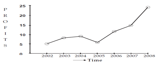
Line graph

­

Line graphs represent the variation of a value over another metric, such as time. In general, values are represented in the vertical axis, while the time variation is represented in the horizontal axis.

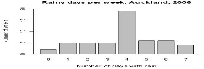
Bar chart

A bar chart is a graph that shows categorical data as bars presenting heights (vertical bar) or widths (horizontal bar) proportional to represent values. Bar charts provide an image that could also be represented in a tabular format.

In the bar chart example, we have the birth rate in Brazil for the December months from 2010 to 2016.The sharp fall in December 2016 reflects the outbreak of Zika virus in the birth rate in Brazil.

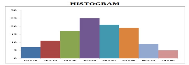
Histograms

The histogram (or frequency distribution) is a graphical representation of a dataset tabulated and divided into uniform or non-uniform classes. It was first introduced by Karl Pearson.

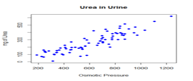
Scatter Plot

A scatter plot is a mathematical diagram that uses Cartesian coordinates to display values of a dataset. A scatter plot shows the data as a set of points, each one presenting the value of one variable determining the position on the horizontal axis and another variable on the vertical axis. They are also called scatter graph, scatter chart, scatter gram, or scatter diagram.

Q4) Define the mean, mode, median, and correlation coefficient?

A4)

Mean

The arithmetic mean is the sum of a collection of values (x1+x2+x3+x4….xn)/n divided by the number of items of this collection (n).

Median

The median is the value in the middle of a dataset.

Mode

 Mode (statistics)

The mode is the value of a set of data that appears most often.

Comparison among mean, median and mode Values = { 2,3,3,3,3,3,4,4,11 }

Box Plot

Box plot is a method for graphically depicting groups of numerical data. The maximum and minimum values are represented by the lines, and the interquartile range (IQR) represent 25–75% of the data. Outliers may be plotted as circles.

Correlation Coefficients

Although correlations between two different kinds of data could be inferred by graphs, such as scatter plot, it is necessary validate this though numerical information. For this reason, correlation coefficients are required. They provide a numerical value that reflects the strength of an association.

Q5) Give brief description about Inferential Statistics.

A5)

It is used to make inferences about an unknown population, by estimation and/or hypothesis testing. In other words, it is desirable to obtain parameters to describe the population of interest, but since the data is limited, it is necessary to make use of a representative sample in order to estimate them. With that, it is possible to test previously defined hypotheses and apply the conclusions to the entire population. The standard error of the mean is a measure of variability that is crucial to do inferences.

Hypothesis testing

Hypothesis testing is essential to make inferences about populations aiming to answer research questions, as settled in "Research planning" section. Authors defined four steps to be set

The hypothesis to be tested: as stated earlier, we have to work with the definition of a null hypothesis (H0), that is going to be tested, and an alternative hypothesis. But they must be defined before the experiment implementation.

Significance level and decision rule: A decision rule depends on the level of significance, or in other words, the acceptable error rate (α). It is easier to think that we define a critical value that determines the statistical significance when a test statistic is compared with it. So, α also has to be predefined before the experiment.

Experiment and statistical analysis: This is when the experiment is really implemented following the appropriate experimental design, data is collected and the more suitable statistical tests are evaluated.

Inference: Is made when the null hypothesis is rejected or not rejected, based on the evidence that the comparison of p-values and α brings. It is pointed that the failure to reject H0 just means that there is not enough evidence to support its rejection, but not that this hypothesis is true.

Q6) What is Statistical Considerations and also define type of error?

A6)

Power and statistical error

When testing a hypothesis, there are two types of statistic errors possible: Type I error and Type II error. The type I error or false positive is the incorrect rejection of a true null hypothesis and the type II error or false negative is the failure to reject a false null hypothesis. The significance level denoted by α is the type I error rate and should be chosen before performing the test. The type II error rate is denoted by β and statistical power of the test is 1 −β.

P -Value 

The p-value is the probability of obtaining results as extreme as or more extreme than those observed, assuming the null hypothesis (H0) is true. It is also called the calculated probability. It is common to confuse the p-value with the significance level (α), but, the α is a predefined threshold for calling significant results. If p is less than α, the null hypothesis (H0) is rejected.

Multiple testing

In multiple tests of the same hypothesis, the probability of the occurrence of falses positives (familywise error rate) increase and some strategy are used to control this occurrence. This is commonly achieved by using a more stringent threshold to reject null hypotheses. The Bonferroni correction defines an acceptable global significance level, denoted by α* and each test is individually compared with a value of α = α*/m. This ensures that the familywise error rate in all m tests, is less than or equal to α*. When m is large, the Bonferroni correction may be overly conservative

Q7) Describe application of biostatics in brief.

A7)

Public health

Public health, including epidemiology, health services research, nutrition, environmental health and health care policy & management. In these medicine contents, it's important to consider the design and analysis of the clinical trials. As one example, there is the assessment of severity state of a patient with a prognosis of an outcome of a disease.

With new technologies and genetics knowledge, biostatistics is now also used for Systems medicine, which consists in a more personalized medicine. For this, is made an integration of data from different sources, including conventional patient data, clinico-pathological parameters, molecular and genetic data as well as data generated by additional new-omics technologies.

Quantitative genetics

The study of Population genetics and Statistical genetics in order to link variation in genotype with a variation in phenotype In other words, it is desirable to discover the genetic basis of a measurable trait, a quantitative trait,that is under polygenic control. A genome region that is responsible for a continuous trait is called Quantitative trait locus (QTL). The study of QTLs become feasible by using molecular markers and measuring traits in populations, but their mapping needs the obtaining of a population from an experimental crossing, like an F2 or Recombinant inbred strains/lines (RILs). To scan for QTLs regions in a genome, a gene map based on linkage have to be built. Some of the best-known QTL mapping algorithms are Interval Mapping, Composite Interval Mapping, and Multiple Interval Mapping.

Expression data

Studies for differential expression of genes from RNA-Seq data, as for RT-qPCR and microarrays, demands comparison of conditions. The goal is to identify genes which have a significant change in abundance between different conditions. Then, experiments are designed appropriately, with replicates for each condition/treatment, randomization and blocking, when necessary. In RNA-Seq, the quantification of expression uses the information of mapped reads that are summarized in some genetic unit, as exons that are part of a gene sequence.

Q8) What is the Hypothesis testing and ANNOVA?

A8)

Hypothesis testing is one of the most important inferential tools of application of statistics to real life problems. It is used when we need to make decisions concerning populations on the basis of only sample information. A variety of statistical tests are used to arrive at these decisions (e.g. Analysis of Variance, Chi-Square Test of Independence, etc.). Steps involved in hypothesis testing include specifying the null (H0) and alternate (Ha or H1) hypotheses; choosing a sample; assessing the evidence; and making conclusions.

1. Choosing a Sample:

I chose the NESARC, a representative sample of 43,093 non-institutionalized adults in the U.S. As I am interested in evaluating these hypotheses only among individuals who are smokers and who are younger (rather than older) adults, I subset the NESARC data to individuals that are 1) current daily smokers (i.e. smoked in the past year CHECK321 ==1, smoked over 100 cigarettes S3AQ1A ==1, typically smoked every day S3AQ3B1 == 1) are 2) between the ages 18 and 25. This sample (n=1320) showed the following:

While it is true that 13.9 cigarettes per day are more than 13.2 cigarettes per day, it is not at all clear that this is a large enough difference to reject the null hypothesis.

2. Assessing the Evidence:

In order to assess whether the data provide strong enough evidence against the null hypothesis (i.e. against the claim that there is no relationship between smoking and depression), we need to ask ourselves: How surprising is it to get a difference of 0.7373626 cigarettes smoked per day between our two groups (depression vs. no depression) assuming that the null hypothesis is true (i.e. there is no relationship between smoking and depression).

The Idea behind the ANOVA F-Tests

Let’s think about how we would go about testing whether the population means µ1,µ2,µ3,µ4 are equal. It seems as if the best we could do is to calculate their point estimates—the sample mean in each of our 4 samples (denote them by ȳ1,ȳ2,ȳ3,ȳ4), and see how far apart these sample means are, or, in other words, measure the variation between the sample means. If we find that the four sample means are not all close together, we’ll say that we have evidence against Ho, and otherwise, if they are close together, we’ll say that we do not have evidence against Ho.

Q9) What is Skewed Distributions and Data Transformation?

A9)

A skewed distribution is neither symmetric nor normal because the data values trail off more sharply on one side than on the other. In business, you often find skewness in data sets that represent sizes using positive numbers (eg, sales or assets). The reason is that data values cannot be less than zero (imposing a boundary on one side) but are not restricted by a definite upper boundary. The result is that there are many data values concentrated near zero, and they become systematically fewer and fewer as you move to the right in the histogram. 

Transformation to the Rescue

One solution to this dilemma of skewness is to use transformation to make a skewed distribution more symmetric. Transformation refers to replacing each data value by a different number (such as its logarithm) to facilitate statistical analysis. The most common transformation in business and economics is the logarithm, which can be used only on positive numbers (ie, if your data include negative numbers or zero, this technique cannot be used). Using the logarithm often transforms skewness into symmetry because it stretches the scale near zero, spreading out all of the small values, which had been bunched together. It also pulls together the very large data values, which had been thinly spread out at the high end.

Q10) What are the applications of mean, mode, median biometrics?

A10)

Application of Mean, Median & Mode